NSDT工具推荐: Three.js AI纹理开发包 - YOLO合成数据生成器 - GLTF/GLB在线编辑 - 3D模型格式在线转换 - 可编程3D场景编辑器 - REVIT导出3D模型插件 - 3D模型语义搜索引擎 - AI模型在线查看 - Three.js虚拟轴心开发包 - 3D模型在线减面 - STL模型在线切割 - 3D道路快速建模
R树是用于空间访问方法的树数据结构,即用于索引多维信息,例如地理坐标、矩形或多边形。
1、空间数据
如果一个对象至少具有一个捕获其在 2D 或 3D 空间中的位置的属性,则该对象被表征为空间对象。 此外,空间物体可能在空间中具有几何范围。 例如,我们可以说建筑物是一个空间对象,因为它在 2D 或 3D 地图中具有位置和几何范围。
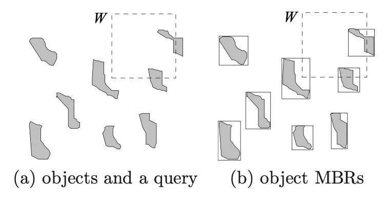
在多维空间中不存在保持空间邻近性的全序。 因此,空间中的对象无法以理论上为空间查询提供最佳性能范围的方式物理集群到磁盘页面。
假设我们尝试使用某些一维排序键对一组二维点进行排序。 无论我们使用哪个键,按皮亚诺曲线或希尔伯特排序的列排序,我们都不能保证任何在空间上接近的对象对在总顺序上也将接近。
R 树正在绘制我们的世界,这是一个现实世界的应用程序。 它们存储空间数据对象,例如商店位置和创建地图的所有其他形状。 例如,从城市街区或您最喜欢的餐厅创建多边形的地理坐标。
为什么这个有用?
嘿,Siri! 找到离我最近的麦当劳
是的,我们需要根据对象的实际位置进行查询。
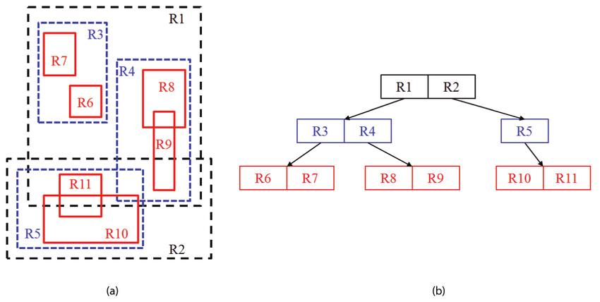
2、R树中的“R”代表矩形
数据结构的关键思想是将附近的对象分组并用矩形表示它们。 最小外接矩形或简称 MBR。 这是递归发生的:
由于所有对象都位于此边界矩形内,因此不与边界矩形相交的查询也无法与任何包含的对象相交。 在叶级别,每个矩形描述一个空间对象。 所有其他级别都只是节点指针。
该树的一个约束是每个节点(根节点除外)应至少为 40%,以便正确利用磁盘空间。 下面我们可以看到 R 树的示例。
为了保持 R 树的利用率,我们必须做四件事:
- 目录节点条目的 MBR 所覆盖的区域应最小化。
- 同一级别目录项的 MBR 之间的重叠应最小化。
- 目录节点条目的 MBR 的边距应最小化。
- R 树节点中的平均条目数应最大化。
3、批量加载
批量加载(bulk loading)是一种通常以“大块”的方式将数据加载到数据库中的方法。 我们将使用一种称为排序平铺递归 (STR:Sort Tile Recursive) 的方法。
每个 MBR 包含以下由制表符 (‘\t’) 分隔的内容: object-id、 x-low、 x-high、 y-low、 y-high。 下面我们可以看到一个计算矩形列表的 MBR 的函数。 每个矩形都存储在一个字符串中:
def find_mbr(slc):

  # convert the string that contains the rectangles info into a list of lists
  a = [item.split() for item in slc]

  # itemgetter(0) has the id

  x_low = min(a, key=operator.itemgetter(1))[1]
  x_max = max(a, key=operator.itemgetter(2))[2]
  y_low = min(a, key=operator.itemgetter(3))[3]
  y_max = max(a, key=operator.itemgetter(4))[4]

  return [x_low, x_max, y_low, y_max]
STR 技术首先根据矩形的 x-low 对 n 个矩形进行排序。 经过排序,我们知道树中会有 L = ⌈n/C⌉ 的叶子节点。 属性C指的是每个节点的容量。 具体来说它可以存储多少个矩形:
def construct(rectangle_file, node_array, counter_left_of):

  global tree_level
  global node_counter


  # sort according to the second column (x-low).
  data = sorted(rectangle_file, key=lambda line: line.split()[1])

  number_of_data_rectangles = len(data)

  # assume each rectangle needs 36 bytes and each node can hold up to 1200 bytes.
  node_can_hold = math.floor(1200 / 36)

  number_of_nodes = math.ceil(number_of_data_rectangles / node_can_hold)

  number_of_slices = math.ceil(math.sqrt(number_of_nodes))
然后,(已排序的)矩形被分为 ⌈SquareRoot( L)⌉ 组(垂直条纹),并且使用矩形的 y-low 作为键对每个组进行排序。 这种排序的输出被打包到叶节点中,并且树是通过递归调用以自下而上的方式构建的。
if number_of_slices > 1:

  # create the slices
  slices = list(divide_chunks(data, node_can_hold*number_of_slices))

  # sort every slice according to the fourth column (y-low)
  sorted_slices = [sorted(item, key=lambda line: line.split()[3]) for item in slices]

  # merges the slices into a single list
  concat_list = [j for i in sorted_slices for j in i]

  # divide them again in chunks that a node can hold

  slices = list(divide_chunks(concat_list, node_can_hold))

  # find the MBR of each slice
  mbr = [find_mbr(item) for item in slices]

  # this counter is passed to the upper recursion level so the
  # next level nodes will know where to point.

  counter_left_of = node_counter

  # append the nodes in the node array

  for slc in slices:
    node_array.append(Node(node_counter, len(slc), slc, tree_level))
    node_counter += 1

  node_ids = [i for i in range(counter_left_of, node_counter)]

  # create the chunks that are needed for the upper level, mbrs of every slice and where
  # they will point

  data_for_the_upper = [str(a) + '\t' + str(b[0]) + '\t' + str(b[1]) + '\t' + str(b[2]) + '\t' + str(b[3]) for
                        a, b in zip(node_ids, mbr)]

  tree_level += 1

  number_of_nodes_per_level.append(number_of_nodes)
  average_MBR_area_per_level.append(get_area(data)/len(data))

  # recursively construct from bottom to top
  construct(data_for_the_upper, node_array, counter_left_of)
当切片数为 1 时,递归结束。这意味着我们到达了根级别:
# recursion is over, we reached top node
else:

  # sort  according to the fourth column (y-low)
  data = sorted(data, key=lambda line: line.split()[4])

  node_array.append(Node(node_counter, len(data), data, tree_level))
  node_counter += 1
4、让我们查询树
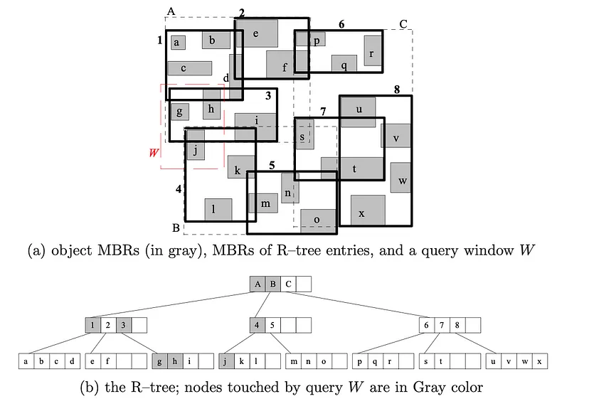
遵循与查询范围相交的条目指针,以深度优先的方式遍历树。 查询算法采用三个参数; 查询范围q,检索对象应满足q的谓词θ,以及R树节点n。
如果我们位于叶节点上,我们会搜索该节点的每个 MBR 以检查它们是否满足我们的查询。 如果是的话,我们将矩形添加到答案集中。
如果我们不在叶节点上,我们将搜索该节点的每个 MBR 以检查它们是否满足我们的查询。 如果确实如此,我们将递归调用该函数。 我们使用相同的参数。 唯一改变的参数是节点。 我们现在正在传递当前节点所指向的节点。
简单来说,我们要检查是否与查询的 MBR 存在交集。
我们希望能够执行 3 种查询类型。 交集,对于至少有一个公共点的 MBR,内部,对于位于查询内部的 MBR,以及包含,对于包含查询的 MBR 的 MBR。
def query(rectangles_answer_set, rectangle_of_the_query, node_array, node_from_recursion, first_call, nodes_accessed,
          q_type):

    # hacky way to count the accesses with a mutable type passing with reference, globals would not work here
    nodes_accessed.append('1')

    if first_call:
        # the first call gets the root node
        node_to_check = node_array[-1]
    else:
        node_to_check = node_from_recursion

    if node_to_check.tree_level == 1:

        for mbr in node_to_check.list_of_attrs:

            mbr_splitted = mbr.split()

            if query_type(rectangle_of_the_query, mbr_splitted, q_type):
                rectangles_answer_set.append(mbr)

    else:

        for mbr in node_to_check.list_of_attrs:
            mbr_splitted = mbr.split()
            points_to = mbr_splitted[0]

            if query_type(rectangle_of_the_query, mbr_splitted, 'intersection'):
                query(rectangles_answer_set, rectangle_of_the_query, node_array, node_array[int(points_to)], False,
                      nodes_accessed, q_type)
每个非叶节点必须仅检查交集。 我们可以通过下面的例子看到,如果我们严格过滤非叶节点上的所有 MBR,我们会错过很多结果。
考虑内部查询和非叶节点处的步骤。 黑色矩形是查询的 MBR。 红色是被过滤的中间节点,绿色是实际对象。 如果在递归中我们有严格的规则要求 MBR 完全位于内部进行检查,则红色将不会通过过滤器,因此我们将失去绿色的 MBR,因为它是符合标准的实际对象:
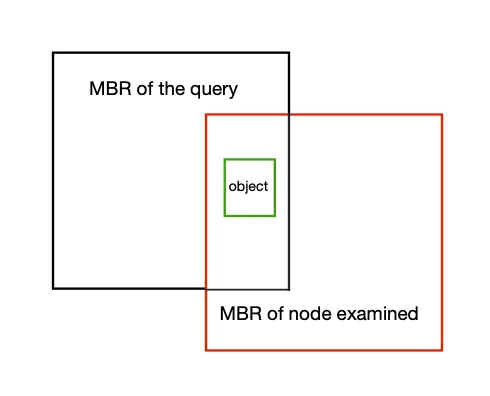
接受对象的标准取决于其几何形状,如下所示:
# At least one  point intersecting.
if q_type == 'intersection':

    x_axis = (query_x_high >= mbr_x_low) or (query_x_high <= mbr_x_high)
    y_axis = (query_y_low <= mbr_y_high) or (query_y_high <= mbr_y_low)

    return x_axis and y_axis

# The MBR of the rectangle we examine must be inside of the MBR of the query.
elif q_type == 'inside':

    x_axis = (query_x_high >= mbr_x_high) and (query_x_low <= mbr_x_low)
    y_axis = (query_y_low <= mbr_y_low) and (query_y_high >= mbr_y_high)

    return x_axis and y_axis

# Exactly the opposite from the previous. We can change the positions in the comparisons.
elif q_type == 'containment':

    x_axis = (mbr_x_high >= query_x_high) and (mbr_x_low <= query_x_low)
    y_axis = (mbr_y_low <= query_y_low) and (mbr_y_high >= query_y_high)

    return x_axis and y_axis
5、结束语
空间数据库系统中处理空间选择的方式取决于所查询的关系 R 是否已索引。 如果 R 没有索引,我们线性扫描它并将每个对象与查询范围进行比较。 正如所讨论的,DBMS 应用了两步处理技术,该技术在对象的精确几何形状之前针对查询测试对象的 MBR。 如果关系被索引(例如,通过 R 树),那么我们可以使用它来快速查找符合过滤步骤的对象。
原文链接:Bulk loading R-trees and how to store higher dimension data
BimAnt翻译整理,转载请标明出处