
NSDT工具推荐: Three.js AI纹理开发包 - YOLO合成数据生成器 - GLTF/GLB在线编辑 - 3D模型格式在线转换 - 可编程3D场景编辑器 - REVIT导出3D模型插件 - 3D模型语义搜索引擎 - AI模型在线查看 - Three.js虚拟轴心开发包 - 3D模型在线减面 - STL模型在线切割 - 3D道路快速建模
从 2D 图像重建 3D 对象是一项非常有趣的任务,并且具有许多实际应用,但实现高质量并将 2D 图像点准确地映射到 3D 世界空间也非常具有挑战性,特别是对于初学者而言。 要了解不同 3D 框架中坐标系的基础知识,在深入研究之前,请查看我们早些时候的文章《掌握 3D 空间:OpenCV、COLMAP、PyTorch3D 和 OpenGL 中坐标系转换的综合指南》。 在本文中,我们将尝试根据 Python 的渲染图像重建斯坦福兔子的 3D 网格。
1、概述
在开始实施之前,让我们先了解一下 3D 重建需要了解的一些主要概念。
1.1 相机的内参和外参
内在参数(intrinsic parameters)是相机的内部参数,例如焦距、主点和镜头畸变。外部参数(extrinsic parameters)定义相机在 3D 空间中的位置和方向。
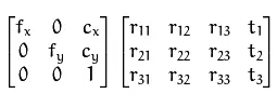
外部矩阵通常保持 4x4 排列,包括 3x3 旋转矩阵和平移向量。 而内在矩阵通常采用 3x3 格式描述焦距和相机投影中心,而在 PyTorch3D 中采用 4x4 形状。
要深入了解相机参数,请参阅阿基尔·安瓦尔的这篇文章 。
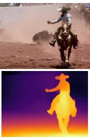
1.2 深度估计
深度估计是计算物体距相机或观察者有多远的过程。 我们将使用 PyTorch3D fragments zbuf 来获取兔子渲染图像的 z 坐标(深度)。 你还可以使用不同的模型来使用相机内在函数(例如 IronDepth 和 MiDaS)来预测图像的深度。
1.3 反向投影
反向投影(back projection)是计算机视觉中的一个过程,其中图像中的 2D 点转换为世界空间中的 3D 坐标。 这涉及使用相机内部参数(焦距、主点)、相机外部参数(旋转和平移)以及 2D 图像中点的深度信息等信息。 通过考虑这些参数,反投影有助于将 2D 图像中的像素映射回现实空间中相应的 3D 位置。
在我们的例子中,我们将使用 PyTorch3D的 unproject_points 函数执行反投影。
1.4 网格
将 3D 计算机图形学中的多边形网格视为对象的虚拟皮肤。 它由称为顶点的点组成,通过称为边的线连接,它们一起形成称为面的平面。 将这些面想象成覆盖物体的小三角形。
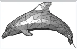
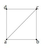
要在 python 中创建面,我们将通过从顶点列表创建上三角形和下三角形来使用三角测量方法。
2、环境设置
首先,下载我创建的 YML 文件,其中列出了完成该项目所需的所有必要包:
name: 3d_env
channels:
  - pytorch3d
  - nvidia/label/cuda-11.8.0
  - intel
  - https://aws-ml-conda-preview.s3.us-west-2.amazonaws.com
  - conda-forge
dependencies:
  - _libgcc_mutex=0.1=conda_forge
  - _openmp_mutex=4.5=2_kmp_llvm
  - aws-ofi-nccl-dlc=1.7.1=aws_0
  - blas=1.0=mkl
  - boto3=1.28.69=pyhd8ed1ab_0
  - botocore=1.31.69=pyhd8ed1ab_0
  - brotli-python=1.1.0=py310hc6cd4ac_1
  - bzip2=1.0.8=h7f98852_4
  - ca-certificates=2023.7.22=hbcca054_0
  - certifi=2023.7.22=pyhd8ed1ab_0
  - charset-normalizer=3.3.1=pyhd8ed1ab_0
  - colorama=0.4.6=pyhd8ed1ab_0
  - cuda-cudart=11.8.89=0
  - cuda-cupti=11.8.87=0
  - cuda-libraries=11.8.0=0
  - cuda-nvrtc=11.8.89=0
  - cuda-nvtx=11.8.86=0
  - cuda-runtime=11.8.0=0
  - dataclasses=0.8=pyhc8e2a94_3
  - dpcpp-cpp-rt=2023.2.0=h59595ed_49500
  - dpcpp_cpp_rt=2023.2.0=intel_49495
  - ffmpeg=4.2=h3fd9d12_1
  - filelock=3.12.4=pyhd8ed1ab_0
  - freetype=2.12.1=h267a509_2
  - fvcore=0.1.5.post20221221=pyhd8ed1ab_0
  - gettext=0.21.1=h27087fc_0
  - gmp=6.2.1=h58526e2_0
  - gmpy2=2.1.2=py310h3ec546c_1
  - gnutls=3.6.15=he1e5248_0
  - hwloc=2.9.2=h2bc3f7f_0
  - icu=73.2=h59595ed_0
  - idna=3.4=pyhd8ed1ab_0
  - intel-cmplr-lib-rt=2023.2.0=hfc55251_49500
  - intel-cmplr-lic-rt=2023.2.0=ha770c72_49500
  - intel-opencl-rt=2023.2.0=heb1d2f6_49500
  - intelpython=2023.2.0=0
  - iopath=0.1.9=pyhd8ed1ab_0
  - jbig=2.1=h7f98852_2003
  - jinja2=3.1.2=pyhd8ed1ab_1
  - jmespath=1.0.1=pyhd8ed1ab_0
  - jpeg=9e=h0b41bf4_3
  - lame=3.100=h166bdaf_1003
  - lcms2=2.12=h3be6417_1
  - ld_impl_linux-64=2.40=h41732ed_0
  - lerc=3.0=h295c915_0
  - libcublas=11.11.3.6=0
  - libcufft=10.9.0.58=0
  - libcufile=1.4.0.31=0
  - libcurand=10.3.0.86=0
  - libcusolver=11.4.1.48=0
  - libcusparse=11.7.5.86=0
  - libdeflate=1.8=h7f8727e_5
  - libffi=3.4.2=h7f98852_5
  - libgcc-ng=13.2.0=h807b86a_2
  - libhwloc=2.9.3=default_h554bfaf_1009
  - libiconv=1.17=h166bdaf_0
  - libidn2=2.3.4=h166bdaf_0
  - libnpp=11.8.0.86=0
  - libnsl=2.0.1=hd590300_0
  - libnvjpeg=11.9.0.86=0
  - libpng=1.6.39=h753d276_0
  - libsqlite=3.43.2=h2797004_0
  - libstdcxx-ng=13.2.0=h7e041cc_2
  - libtasn1=4.19.0=h166bdaf_0
  - libtiff=4.3.0=h6f004c6_2
  - libunistring=0.9.10=h7f98852_0
  - libuuid=2.38.1=h0b41bf4_0
  - libwebp-base=1.3.2=hd590300_0
  - libxml2=2.11.5=h232c23b_1
  - libzlib=1.2.13=hd590300_5
  - llvm-openmp=17.0.3=h4dfa4b3_0
  - markupsafe=2.1.3=py310h2372a71_1
  - mkl=2023.2.0=h84fe81f_50495
  - mkl-service=2.4.0=py310hae59892_35
  - mkl_fft=1.3.6=py310h173b8ae_56
  - mkl_random=1.2.2=py310h1595b48_76
  - mkl_umath=0.1.1=py310hd987cd3_86
  - mpc=1.3.1=hfe3b2da_0
  - mpfr=4.2.1=h9458935_0
  - mpmath=1.3.0=pyhd8ed1ab_0
  - ncurses=6.4=hcb278e6_0
  - nettle=3.7.3=hbbd107a_1
  - networkx=3.2=pyhd8ed1ab_1
  - numpy=1.24.3=py310hed7eef7_0
  - numpy-base=1.24.3=py310he88ecf9_0
  - ocl-icd=2.3.1=h7f98852_0
  - olefile=0.46=pyh9f0ad1d_1
  - openh264=2.1.1=h780b84a_0
  - openjpeg=2.5.0=h7d73246_0
  - openssl=3.1.4=hd590300_0
  - pillow=8.4.0=py310h07f4688_0
  - pip=23.3.1=pyhd8ed1ab_0
  - portalocker=2.8.2=py310hff52083_1
  - pysocks=1.7.1=pyha2e5f31_6
  - python=3.10.12=hd12c33a_0_cpython
  - python-dateutil=2.8.2=pyhd8ed1ab_0
  - python_abi=3.10=4_cp310
  - pytorch=2.0.1=aws_py3.10_cuda11.8_cudnn8.7.0_0
  - pytorch-cuda=11.8=h7e8668a_3
  - pytorch-mutex=1.0=cuda
  - pytorch3d=0.7.4=py310_cu118_pyt201
  - pyyaml=6.0.1=py310h2372a71_1
  - readline=8.2=h8228510_1
  - requests=2.31.0=pyhd8ed1ab_0
  - s3transfer=0.7.0=pyhd8ed1ab_0
  - setuptools=68.2.2=pyhd8ed1ab_0
  - six=1.16.0=pyh6c4a22f_0
  - sympy=1.12=pypyh9d50eac_103
  - tabulate=0.9.0=pyhd8ed1ab_1
  - tbb=2021.10.0=h00ab1b0_2
  - tbb4py=2021.10.0=py310hf5d52d3_2
  - termcolor=2.3.0=pyhd8ed1ab_0
  - tk=8.6.13=h2797004_0
  - torchtriton=2.0.0=py310
  - torchvision=0.15.2=py310_cu118
  - tqdm=4.66.1=pyhd8ed1ab_0
  - typing_extensions=4.8.0=pyha770c72_0
  - tzdata=2023c=h71feb2d_0
  - urllib3=1.26.18=pyhd8ed1ab_0
  - wheel=0.41.2=pyhd8ed1ab_0
  - xz=5.2.6=h166bdaf_0
  - yacs=0.1.8=pyhd8ed1ab_0
  - yaml=0.2.5=h7f98852_2
  - zlib=1.2.13=hd590300_5
  - zstd=1.5.5=hfc55251_0
  - pip:
      - ansi2html==1.8.0
      - asttokens==2.4.0
      - attrs==23.1.0
      - backcall==0.2.0
      - beautifulsoup4==4.12.2
      - click==8.1.7
      - comm==0.1.4
      - configargparse==1.7
      - contourpy==1.1.1
      - cycler==0.12.1
      - dash==2.14.0
      - dash-core-components==2.0.0
      - dash-html-components==2.0.0
      - dash-table==5.0.0
      - debugpy==1.8.0
      - decorator==5.1.1
      - exceptiongroup==1.1.3
      - executing==2.0.0
      - fastjsonschema==2.18.1
      - flask==2.2.5
      - fonttools==4.43.1
      - gdown==4.7.1
      - importlib-metadata==6.8.0
      - ipykernel==6.26.0
      - ipython==8.16.1
      - itsdangerous==2.1.2
      - jedi==0.19.1
      - jsonschema==4.19.1
      - jsonschema-specifications==2023.7.1
      - jupyter-client==8.5.0
      - jupyter-core==5.4.0
      - kiwisolver==1.4.5
      - matplotlib==3.8.0
      - matplotlib-inline==0.1.6
      - nbformat==5.7.0
      - nest-asyncio==1.5.8
      - https://github.com/cubao/Open3D/releases/download/v0.17.0-wheels/open3d_cpu-0.17.0-cp310-cp310-manylinux_2_17_x86_64.whl
      - opencv-python==4.8.1.78
      - packaging==23.2
      - parso==0.8.3
      - pexpect==4.8.0
      - pickleshare==0.7.5
      - platformdirs==3.11.0
      - plotly==5.17.0
      - plyfile==1.0.1
      - prompt-toolkit==3.0.39
      - psutil==5.9.6
      - ptyprocess==0.7.0
      - pure-eval==0.2.2
      - pygments==2.16.1
      - pyparsing==3.1.1
      - pyzmq==25.1.1
      - referencing==0.30.2
      - retrying==1.3.4
      - rpds-py==0.10.6
      - soupsieve==2.5
      - stack-data==0.6.3
      - tenacity==8.2.3
      - tornado==6.3.3
      - traitlets==5.12.0
      - wcwidth==0.2.8
      - werkzeug==2.2.3
      - zipp==3.17.0
      - trimesh==4.0.4
      - ipywidgets==8.1.1
      - k3d==2.16.0
      - diffusers==0.24.0
      - transformers==4.35.2
      - accelerate==0.25.0
我们使用配备 GPU 的 AWS SageMaker 笔记本实例。 根据你的系统要求,可能需要调整某些软件包。 例如,如果你使用的是 CPU,请安装与 CPU 兼容的 PyTorch3D 版本,而不是支持 GPU 的版本。
创建环境:下载后,打开命令行界面并导航到包含 YML 文件的目录。 使用以下命令创建一个新环境:
conda env create -f environment.yml激活环境:创建后,激活新环境:
conda activate 3d_env验证安装:要确保所有软件包均已正确安装,请列出它们:
conda list3、代码工作流程
我们的方法涉及以下关键步骤:
- 加载 bunny兔子的obj 文件并以固定半径定义兔子周围的多个摄像机位置。
- 渲染网格以生成 2D 图像。
- 估计每个图像的深度。
- 使用深度值将 2D 图像反投影到世界空间中。
- 将世界空间中的点三角剖分为顶点和面。
3.1 导入依赖包
import os
import json
import torch
import trimesh
import numpy as np
import open3d as o3d
from tqdm import tqdm
from PIL import Image
from typing import Callable, List, Optional, Tuple
from pytorch3d.io import load_objs_as_meshes, load_obj

import pytorch3d
from pytorch3d.structures import Meshes
import pytorch3d.utils
from pytorch3d.renderer import (
    FoVPerspectiveCameras,
    PointLights,
    Materials,
    RasterizationSettings,
    MeshRenderer,
    MeshRasterizer,
    HardPhongShader,
    TexturesUV,
    TexturesVertex,
    Textures
)
3.2 设置计算设备
if torch.cuda.is_available():
    device = torch.device("cuda:0")
    torch.cuda.set_device(device)
else:
    device = torch.device("cpu")
3.3 渲染参数设置
在此代码片段中,我们设置渲染 3D 模型的基本参数:
# Configuring Rendering Parameters
img_resolution = (256, 256)

raster_settings = RasterizationSettings(
    image_size=img_resolution,
    bin_size=None,
    blur_radius=0.0,
    faces_per_pixel=1,
)

lights = PointLights(device=device, location=[[-2.0, -2.0, -5.0]])

materials = Materials(
    device=device,
    specular_color=[[0.0, 0.0, 0.0]],
    shininess=0.0
)

rasterizer=MeshRasterizer(raster_settings=raster_settings)

# Set up a renderer.
renderer = MeshRenderer(
    rasterizer=rasterizer,
    shader=HardPhongShader(device=device, lights=lights)
)- 图像分辨率:定义渲染图像的大小。
- 光栅化设置:确定网格如何转换为 2D 图像,包括模糊半径和每像素面等细节。
- 照明和材质:配置照明和材质属性,这会影响光线与 3D 模型表面的交互方式。
- 光栅化器和渲染器:光栅化器将 3D 网格转换为 2D 图像,渲染器根据定义的设置应用照明和着色效果。
3.4 加载和准备网格
设置渲染环境后,下一步是加载并准备斯坦福兔子的 3D 网格。 此过程包括读取网格数据、对其进行标准化以及设置其纹理。
def load_mesh(obj_file_path, device="cuda"):
    mesh = load_objs_as_meshes([obj_file_path], device=device)
    verts, faces = mesh.get_mesh_verts_faces(0)
    texture_rgb = torch.ones_like(verts, device=device)
    texture_rgb[:, 1:] *= 0.0  # red, by zeroing G and B
    mesh.textures = Textures(verts_rgb=texture_rgb[None])

    # Normalize mesh
    verts = verts - verts.mean(dim=0)
    verts /= verts.max()

    # This updates the pytorch3d mesh with the new vertex coordinates.
    mesh = mesh.update_padded(verts.unsqueeze(0))
    verts, faces = mesh.get_mesh_verts_faces(0)

return mesh, verts, faces - 加载网格:
load_objs_as_meshes函数读取包含Stanford Bunny 网格的OBJ 文件并将其加载到指定设备(GPU 或CPU)上。 - 纹理分配:创建统一的纹理并将其分配给网格。 在本例中,它是红色纹理,通过将绿色和蓝色通道归零来实现。
- 网格归一化:归一化网格的顶点可确保其适当居中和缩放,这对于一致的渲染和重建至关重要。
- 更新网格:使用归一化后的新顶点坐标更新网格对象。
mesh_file_path = "stanford-bunny.obj"
mesh, verts, faces = load_mesh(mesh_file_path)

print(
    f"Loaded Mesh from : {mesh_file_path}"
    f"\nVertices: {verts.shape}"
    f"\nFaces: {faces.shape}"
)- 加载网格:使用斯坦福兔子 OBJ 文件的路径调用
load_mesh函数。 该函数返回网格及其顶点和面。 - 输出信息:打印语句确认网格加载成功。 它还提供有关网格中顶点和面数量的信息。
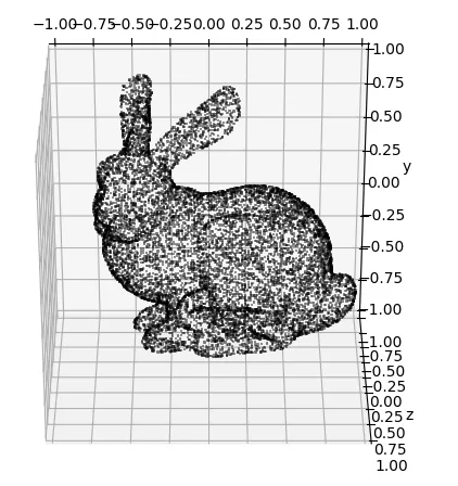
3.5 将网格可视化为点云
加载网格后,有用的下一步是将其可视化以确认其结构和完整性。 这是通过将顶点绘制为点云来完成的,提供网格的视觉表示。
def plot_pointcloud(
    vertices,
    alpha=.5,
    title=None,
    max_points=10_000,
    xlim=(-1, 1),
    ylim=(-1, 1),
    zlim=(-1, 1)
    ):
    """Plot a pointcloud tensor of shape (N, coordinates)
    """
    vertices = vertices.cpu()

    assert len(vertices.shape) == 2
    N, dim = vertices.shape
    assert dim==2 or dim==3

    if N > max_points:
        vertices = np.random.default_rng().choice(vertices, max_points, replace=False)
    fig = plt.figure(figsize=(6,6))
    if dim == 2:
        ax = fig.add_subplot(111)
    elif dim == 3:
        ax = fig.add_subplot(111, projection='3d')
        ax.set_zlabel("z")
        ax.set_zlim(zlim)
        ax.view_init(elev=120., azim=270)

    ax.set_xlabel("x")
    ax.set_ylabel("y")

    ax.set_xlim(xlim)
    ax.set_ylim(ylim)

    ax.scatter(*vertices.T, alpha=alpha, marker=',', lw=.5, s=1, color='black')
    plt.show(fig)


plot_pointcloud(verts)- 函数定义:
plot_pointcloud获取网格的顶点并绘制它们。alpha、max_points和轴限制(xlim, ylim, zlim)等参数控制绘图的外观。 - 处理大点集:如果顶点数量超过
max_points,则会选择随机子集以保持绘图易于管理且清晰。 - 绘图:该函数根据输入顶点的维数以 2D 或 3D 方式绘图。 它使用 Matplotlib 进行可视化。
- 可视化兔子网格:最后,使用斯坦福兔子网格的顶点调用
plot_pointcloud,从而产生点云的可视化表示。
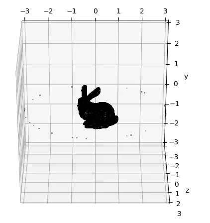
3.6 相机位置和组合可视化
网格成功可视化后,下一个代码片段将模拟摄像机位置添加到场景中。 这些相机点对于从不同角度渲染网格以进行 3D 重建至关重要。
mesh_center = torch.tensor([0.0, 0.0, 0.0], device=device)

points = generate_camera_locations(mesh_center, 3, 100)

plot_pointcloud(torch.cat((points, verts), dim=0), xlim=(-3, 3), ylim=(-3, 3), zlim=(-3, 3))- 网格中心:我们定义一个点,
mesh_center,作为在网格周围生成相机位置的参考。 - 相机位置:
generate_camera_locations函数在mesh_center周围创建一组呈球形分布的点。 指定了点的数量(在本例中为 100),代表不同的摄像机视图。 - 组合绘图:然后使用
plot_pointcloud函数绘制Stanford Bunny 网格的顶点(顶点)和相机位置(点)。 该组合图不仅有助于可视化网格,还有助于可视化 3D 空间中摄像机的相对位置。
3.7 设置相机视图
此片段对于设置从生成的相机位置“查看”网格的相机视图至关重要,确保我们的虚拟相机瞄准网格中心以实现最佳渲染。
R_pt3d, T_pt3d = get_look_at_views(points, mesh_center.repeat(points.shape[0], 1))- 旋转和平移矩阵:
get_look_at_views函数计算每个摄像机位置的旋转 (R_pt3d) 和平移 (T_pt3d) 矩阵,以便每个摄像机面向网格中心。 - 目标点复制:
mesh_center.repeat(points.shape[0], 1)复制每个摄像机点的网格中心坐标,确保所有摄像机都指向网格的同一中心点。
3.8 定义相机本质
以下代码片段指定了相机的内在参数,这对于从 3D 网格渲染 2D 图像至关重要。 这些参数包括焦距、主点和其他相机特定的特性。
K_pt3d = torch.tensor([[0.7, 0., 0.5, 0.],
                        [0., 0.7, 0.5, 0.],
                        [0., 0., 0., 1.0],
[0., 0., 1., 0.]], device=device)- 矩阵
K_pt3d:该张量表示相机的固有矩阵,其中包括: - 沿 x 轴和 y 轴的焦距(本例中为 0.7)。相机的光学中心,通常假设位于图像的中心(此处为 0.5,0.5)。
- 最后一行特定于射影变换中使用的齐次坐标。
3.9 标准化像素坐标生成
在进入主重建流程之前,我们需要准备用于将 2D 图像像素反投影到 3D 空间的像素坐标。
def get_normalized_pixel_coordinates_pt3d(
    y_resolution: int,
    x_resolution: int,
    device: torch.device = torch.device('cpu')
):
    """For an image with y_resolution and x_resolution, return a tensor of pixel coordinates
    normalized to lie in [0, 1], with the origin (0, 0) in the bottom left corner,
    the x-axis pointing right, and the y-axis pointing up. The top right corner
    being at (1, 1).

    Returns:
        xy_pix: a meshgrid of values from [0, 1] of shape
                (y_resolution, x_resolution, 2)
    """
    xs = torch.linspace(1, 0, steps=x_resolution)  # Inverted the order for x-coordinates
    ys = torch.linspace(1, 0, steps=y_resolution)  # Inverted the order for y-coordinates
    x, y = torch.meshgrid(xs, ys, indexing='xy')
return torch.cat([x.unsqueeze(dim=2), y.unsqueeze(dim=2)], dim=2).to(device)- 函数定义:
get_normalized_pixel_coordinates_pt3d为具有给定分辨率的图像创建归一化像素坐标张量。 坐标标准化为范围[0, 1]。 - 轴反转:该函数反转 x 和 y 坐标的顺序,因为在许多图像处理上下文中,原点 (0,0) 位于左上角,但我们将其设置在左下角,右上角为 ( 1, 1) 遵循 PyTorch3D 格式。
- 以下是我们在整个项目中必须遵循的一些主要 PyTorch3D 格式要求:1:内参矩阵的形状应为 [4, 4],而不是 [3, 3]。2:PyTorch3D 将输入作为行向量进行乘法。 因此,在传递给 PyTorch3D 预定义方法之前,请先转置姿势矩阵。
- 通过阅读 掌握 3D 空间,了解有关主要 3D 工具以及如何将输入转换为正确格式的更多信息。
- 网格栅格创建:它使用
torch.meshgrid创建一个由 x 和 y 值组成的网格,这些网格对应于图像上的标准化像素位置。 - 张量串联:x 和 y 坐标连接并扩展为二维网格,形成 3D 张量,其中每个像素位置由一对值 (x, y) 表示。
- 设备分配:将生成的张量移动到指定设备(默认为 CPU,但可以设置为 GPU 以加快计算速度)。
3.10 网格清理
clean_mesh 函数是一个综合实用程序,可清理和细化 3D 重建过程中生成的网格。 此步骤对于确保最终网格具有高质量且没有常见的几何伪影至关重要。
def clean_mesh(vertices: torch.Tensor, faces: torch.Tensor, edge_threshold: float = 0.1, min_triangles_connected: int = -1, fill_holes: bool = True) -> (torch.Tensor, torch.Tensor, torch.Tensor):
    """
    Performs the following steps to clean the mesh:

    1. edge_threshold_filter
    2. remove_duplicated_vertices, remove_duplicated_triangles, remove_degenerate_triangles
    3. remove small connected components
    4. remove_unreferenced_vertices
    5. fill_holes

    :param vertices: (3, N) torch.Tensor of type torch.float32
    :param faces: (3, M) torch.Tensor of type torch.long
    :param colors: (3, N) torch.Tensor of type torch.float32 in range (0...1) giving RGB colors per vertex
    :param edge_threshold: maximum length per edge (otherwise removes that face). If <=0, will not do this filtering
    :param min_triangles_connected: minimum number of triangles in a connected component (otherwise removes those faces). If <=0, will not do this filtering
    :param fill_holes: If true, will perform trimesh fill_holes step, otherwise not.

    :return: (vertices, faces, colors) tuple as torch.Tensors of similar shape and type
    """
    if edge_threshold > 0:
        # remove long edges
        faces = edge_threshold_filter(vertices, faces, edge_threshold)

    # cleanup via open3d
    mesh = torch_to_o3d_mesh(vertices, faces) #, colors)
    mesh.remove_duplicated_vertices()
    mesh.remove_duplicated_triangles()
    mesh.remove_degenerate_triangles()

    if min_triangles_connected > 0:
        # remove small components via open3d
        triangle_clusters, cluster_n_triangles, cluster_area = mesh.cluster_connected_triangles()
        triangle_clusters = np.asarray(triangle_clusters)
        cluster_n_triangles = np.asarray(cluster_n_triangles)
        triangles_to_remove = cluster_n_triangles[triangle_clusters] < min_triangles_connected
        mesh.remove_triangles_by_mask(triangles_to_remove)

    # cleanup via open3d
    mesh.remove_unreferenced_vertices()

    if fill_holes:
        # misc cleanups via trimesh
        mesh = o3d_to_trimesh(mesh)
        mesh.process()
        mesh.fill_holes()
return mesh- 边阈值:删除边缘长于指定阈值的面,有助于消除不切实际的三角形。
- 删除重复三角形:使用 Open3D,该函数可以删除重复的顶点和三角形以及退化三角形,这些三角形的面积非常小,可能会导致渲染问题。
- 删除小组件:消除可能远离主网格或代表噪声的小而孤立的三角形组。
- 未引用的顶点:删除不属于任何三角形的顶点,清理数据结构。
- 填充孔:这是一个可选步骤,使用 Trimesh 填充网格中的任何孔,使其防水并且更适合 3D 打印或模拟等某些应用。
3.11 点云网格三角剖分
此函数是 3D 重建过程的关键,因为它从深度信息派生的点云创建网格。 它使用图像结构将点三角化为面以形成网格。
def get_mesh(world_space_points, depth, H, W):
    # define vertex_ids for triangulation
    '''
    00---01
    |    |
    10---11
    '''
    vertex_ids = torch.arange(H*W).reshape(H, W).to(depth.device)
    vertex_00 = remapped_vertex_00 = vertex_ids[:H-1, :W-1]
    vertex_01 = remapped_vertex_01 = (remapped_vertex_00 + 1)
    vertex_10 = remapped_vertex_10 = (remapped_vertex_00 + W)
    vertex_11 = remapped_vertex_11 = (remapped_vertex_00 + W + 1)


    # triangulation: upper-left and lower-right triangles from image structure
    faces_upper_left_triangle = torch.stack(
        [remapped_vertex_00.flatten(), remapped_vertex_10.flatten(), remapped_vertex_01.flatten()],  # counter-clockwise orientation
        dim=0
    )
    faces_lower_right_triangle = torch.stack(
        [remapped_vertex_10.flatten(), remapped_vertex_11.flatten(), remapped_vertex_01.flatten()],  # counter-clockwise orientation
        dim=0
    )

    # filter faces with -1 vertices and combine
    mask_upper_left = torch.all(faces_upper_left_triangle >= 0, dim=0)
    faces_upper_left_triangle = faces_upper_left_triangle[:, mask_upper_left]
    mask_lower_right = torch.all(faces_lower_right_triangle >= 0, dim=0)
    faces_lower_right_triangle = faces_lower_right_triangle[:, mask_lower_right]
    faces = torch.cat([faces_upper_left_triangle, faces_lower_right_triangle], dim=1)

    # clean mesh
    mesh = clean_mesh(
        vertices=world_space_points,
        faces=faces,
    )

    return mesh
3.12 3D 网格重建
在主重建流程中,几个关键实用函数 get_normalized_pixel_coordinates_pt3d、 clean_mesh 和 get_mesh 已用于准备数据、细化网格质量并确保准确的三角测量。 主要重建脚本集成了这些实用程序,将 2D 图像转换为紧密结合的 3D 网格。
# Reconstruction
image_size = torch.tensor([img_resolution])
K = K_pt3d.unsqueeze(0)
all_meshes = list()
for idx in tqdm(range(len(points)), desc="Processing meshes"):
# Initialize matrices
R = R_pt3d[idx].unsqueeze(0)
T = T_pt3d[idx].unsqueeze(0)
# Define Camera
cam = pytorch3d.renderer.cameras.PerspectiveCameras(
R=R,
T=T,
K=K,
in_ndc=False,
image_size=[(1,1)],
device=device
)
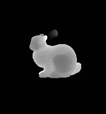
# Render image
images = renderer(mesh, cameras=cam, lights=lights)
image = images[0]
# Depth
fragments = rasterizer(mesh, cameras=cam)
depths = fragments.zbuf
depth = depths[0]
#Back-Projection
xy_pix = get_normalized_pixel_coordinates_pt3d(img_resolution[0], img_resolution[1], device=device)
xy_pix = xy_pix.flatten(0, -2)
depth = depth.flatten(0, -2)
xyz = torch.cat((xy_pix, depth), dim=1)
world_points = cam.unproject_points(xyz)
# Replacing Nan with zeros
world_points = torch.where(torch.isnan(world_points), torch.zeros_like(world_points), world_points)
world_points = world_points[depth.squeeze()!=-1, :]
num_points, _ = world_points.shape
H = int((num_points + 1) ** 0.5)
W = int(num_points / H)
# Triangulation
triangulated_mesh = get_mesh(world_space_points=world_points.T, depth=depth, H=H, W=W)
# Append Mesh
all_meshes.append(triangulated_mesh)image_size:定义图像渲染的分辨率。K:扩展相机内部矩阵以包含批量维度,为多个视图做好准备。all_meshes:初始化为存储每个摄像机视点的重建网格的列表。
循环遍历相机点:
R、T:检索并重塑每个相机视点的旋转和平移矩阵,以适应批处理格式。cam:使用给定的旋转、平移和相机内在函数从 PyTorch3D 初始化PerspectiveCameras对象,定义虚拟相机。images:应用预定义的照明和相机设置,为每个相机视图渲染网格。image:从渲染批次中选择第一张图像进行深度提取。

fragments:栅格化网格以获得片段,其中包括深度缓冲区等。depths:从片段中提取 z 缓冲区(深度值)。depth:检索用于反投影的第一张图像的深度缓冲区。
反投影过程:
- 标准化像素坐标 (
xy_pix):使用get_normalized_pixel_coordinates_pt3d创建并标准化像素坐标网格,确保从 2D 到 3D 的统一映射。 - 展平坐标(
xy_pix和depth):展平 2D 坐标网格并将其与深度值对齐,以实现高效的数据配对。 - 创建 3D 坐标 (
xyz):将 2D 坐标与深度相结合,在相机坐标系中形成 3D 点。 - 世界空间变换 (
world_points):使用unproject_points函数,我们将这些 3D 点从相机坐标转换为世界坐标,将每个点放置在真实世界的 3D 上下文中。
处理无效点(可选):
world_points:处理数据以替换 NaN 值并删除具有无效深度信息的点。 这种删除至关重要,因为负深度通常表示背景元素。 通过过滤掉这些值,我们只关注目标对象的点,提高重建网格的准确性,并确保对象与其背景之间的区别更清晰。
三角化准备:
H、W:根据点数计算点云图像的高度和宽度。triangulated_mesh:使用get_mesh函数对点云进行三角剖分并构建网格。
最终确定:
all_meshes:将每个新重建的网格附加到网格列表中。
该代码通过渲染不同摄像机角度的 2D 图像、提取深度信息、将其转换为 3D 世界坐标,然后从这些点重建网格来完成 3D 重建。 每个步骤对于从 2D 图像创建详细且准确的 3D 网格至关重要。
3.13 网格简化
以下函数用于使用顶点聚类来简化 3D 网格。 此过程对于降低网格的复杂性同时保留其整体形状和特征至关重要。
def simplify_mesh(mesh):
    voxel_size = 0.02
    device = "cuda"
    v = mesh.vertices
    f = mesh.faces
    dtype_v = v.dtype
    dtype_f = f.dtype
    m = o3d.geometry.TriangleMesh()
    m.vertices      = o3d.utility.Vector3dVector(v.astype(np.float64))
    m.triangles     = o3d.utility.Vector3iVector(f.astype(np.int32  ))
    m = m.simplify_vertex_clustering(voxel_size=voxel_size)
    v = np.asarray(m.vertices     ).astype(dtype_v)
    f = np.asarray(m.triangles    ).astype(dtype_f)
    v = torch.from_numpy(v).to(device=device)
    f = torch.from_numpy(f).to(device=device)

    mesh = trimesh.Trimesh(
        vertices = v.cpu(),
        faces = f.cpu()
    )
return meshvoxel_size:体素大小,设置用于顶点聚类的体素大小,确定简化程度。device:设备设置,指定用于计算的设备(例如,GPU 的 CUDA)。vertices和faces:提取输入网格的顶点 (v) 和面 (f) 及其数据类型。- Open3D 网格转换:将网格转换为 Open3D 的 TriangleMesh 格式进行处理。
- 网格简化:使用指定的
voxel_size应用顶点聚类简化。 该技术对每个体素内的顶点进行分组,有效地减少了顶点数量并简化了网格。 - 重新转换为原始格式:将简化的网格转换回 numpy 数组,然后转换为 PyTorch 张量,保持原始数据类型。
- 修剪网格重建:使用修剪网格重建简化的网格以供进一步使用或可视化,确保与管道其他部分的兼容性。
3.14 网格合并功能
此代码片段提供了将两个单独的 3D 网格合并为单个网格的功能。 这在需要将来自不同视点的多个重建网格组合成统一模型的场景中特别有用。
def merge_mesh(mesh1, mesh2):
    v1 = torch.tensor(mesh1.vertices)
    f1 = torch.tensor(mesh1.faces)

    v2 = torch.tensor(mesh2.vertices)
    f2 = torch.tensor(mesh2.faces)

    v = torch.cat([v1, v2], dim=0)
    f = torch.cat([f1, f2 + len(v1)], dim=0)

    merged_mesh = trimesh.Trimesh(
        vertices = v.cpu().numpy(),
        faces = f.cpu().numpy()
    )

return merged_mesh- 顶点和面提取:从两个输入网格中提取顶点(v1,v2)和面(f1,f2)。
- 连接:连接两个网格 (v) 的顶点,并调整第二个网格 (f2) 的面索引,以在连接面之前与新的组合顶点列表对齐。
- 新网格创建:使用组合的顶点和面构造一个新的 Trimesh 对象,从而生成合并的网格。
- Return Merged Mesh:输出最终的合并网格。
3.15 使用管道中的函数
定义合并函数后,代码使用它来组合存储在 all_meshes 中的所有重建网格:
# save combined mesh
mesh_combined = all_meshes[0]
for current_mesh in all_meshes[1:]:
    mesh_combined = merge_mesh(mesh_combined, current_mesh)
    # Optional simplification step
    # mesh_combined = simplify_mesh(mesh_combined)

save_mesh(mesh_combined, "outputs/combined_mesh.ply")- 初始网格设置:从第一个网格开始作为组合的基础。
- 迭代合并:循环遍历剩余网格,将每个网格按顺序与组合网格合并。
- 可选简化:每次合并后都有一个简化网格的选项。 这可以减小整体网格尺寸,但也可能影响网格的细节级别。
- 保存最终网格:最终组合网格保存到指定文件中,提供从多个网格导出的完整 3D 表示。
4、最终的3D 网格
最终的网格显示了斯坦福兔子从侧面的清晰视图,我们放置了相机。 然而,兔子顶部和底部的一些部分缺失了。 发生这种情况是因为我们在成像过程中没有从上方或下方观察的相机。
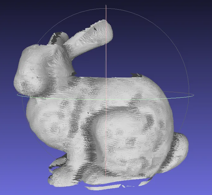
为了解决兔子顶部和底部视图缺失的问题,可以应用两个关键解决方案:
- 在物体上方和下方添加摄像头以获得更好的覆盖范围。
- 使用扩散模型或修复等先进技术来估计和填充未观察区域的外观,从而实现更完整的 3D 重建。
5、结束语
我们对斯坦福兔子的 3D 网格重建凸显了使用多个侧视摄像头进行准确模型生成的潜力。 虽然我们在捕捉兔子的轮廓方面取得了令人印象深刻的成果,但缺乏上方和下方的视图对实现完全封闭的 3D 模型构成了重大挑战。 为了解决这一限制,我们讨论了两种有价值的解决方案:扩大相机覆盖范围以包括缺失的角度或利用扩散模型和修复等先进技术。 这些方法提高了 3D 重建的准确性和全面性。
常见陷阱列举如下:
- 缩放问题:确保所有输入点、相机固有矩阵、像素网格和深度数据一致缩放,以防止可能影响重建质量的缩放问题。
- 覆盖不完整:一个常见的陷阱是仅依赖侧视摄像头,导致重建时丢失细节。
- 数据质量:图像质量差或校准问题可能会导致深度信息不准确并影响最终的网格。
- 后处理复杂性:应用扩散模型等先进技术需要专业知识和计算资源。
- 坐标系一致性:确保您遵循您所使用的框架首选的相同坐标约定或格式。 了解 OpenCV、PyTorch3D、COLMAP 和 OpenGL 使用的坐标系之间的差异和转换对于准确的 3D 重建至关重要。
对于那些有兴趣进一步探索代码的人,你可以在我们的 GitHub 存储库上找到完整的实现代码。
原文链接:Beyond the Surface: Advanced 3D Mesh Generation from 2D Images in Python
BimAnt翻译整理,转载请标明出处


