Open3D模型处理实战

NSDT工具推荐： Three.js AI纹理开发包 - YOLO合成数据生成器 - GLTF/GLB在线编辑 - 3D模型格式在线转换 - 可编程3D场景编辑器 - REVIT导出3D模型插件 - 3D模型语义搜索引擎 - Three.js虚拟轴心开发包 - 3D模型在线减面 - STL模型在线切割

在本文中，我们将学习如何使用 Python 的 Open3D 库探索、处理和可视化 3D 模型。

如果你正在考虑为特定任务处理 3D 数据/模型，例如为 3D 模型分类和/或分割训练 AI 模型，可能会发现本演练很有帮助。在 Internet 上找到的 3D 模型（在 ShapeNet 等数据集中）有多种格式，例如 .obj、.glb、.gltf 等。使用像 Open3D 这样的库，这样的模型可以很容易地处理、可视化并转换成其他格式，比如点云，这些格式更容易理解和解释。

对于那些希望跟随并在本地运行代码的人，本文还可以作为 Jupyter Notebook 使用。包含 Jupyter Notebook 以及所有其他数据和资产的 zip 文件可以从这里下载。

0、开发环境准备

让我们从导入所有必要的库开始：

# Importing open3d and all other necessary libraries.

import open3d as o3d
import os
import copy
import numpy as np
import pandas as pd
from PIL import Image

np.random.seed(42)

# Checking the installed version on open3d.

o3d.__version__
# Open3D version used in this exercise: 0.16.0

1、加载 3D 模型并可视化

通过运行以下代码行，可以将 3D 模型读取为网格：

# Defining the path to the 3D model file.
mesh_path = "data/3d_model.obj"

# Reading the 3D model file as a 3D mesh using open3d.
mesh = o3d.io.read_triangle_mesh(mesh_path)

要可视化网格，请运行以下代码行：

# Visualizing the mesh.
draw_geoms_list = [mesh]
o3d.visualization.draw_geometries(draw_geoms_list)

网格应该会在新窗口中打开，并且应该如下图所示（请注意，网格打开时是静态图像，而不是此处显示的动画图像）。可以使用鼠标指针根据需要旋转网格图像。

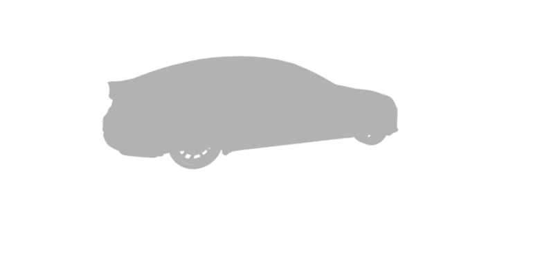
如上所示，汽车网格看起来不像典型的 3D 模型，而是涂成统一的灰色。这是因为网格没有任何关于 3D 模型中顶点和表面法线的信息。

什么是法线？ — 曲面在给定点的法向量是在该点垂直于曲面的向量。法线向量通常简称为“法线”。要阅读有关此主题的更多信息，可以参考这两个链接：Normal Vector 和 Estimating Surface Normals in a PointCloud。

上面 3D 网格的法线可以通过运行以下代码行来估算：

# Computing the normals for the mesh.
mesh.compute_vertex_normals()

# Visualizing the mesh.
draw_geoms_list = [mesh]
o3d.visualization.draw_geometries(draw_geoms_list)

可视化后，网格现在应如下图所示。计算法线后，汽车正确渲染，看起来像一个 3D 模型。

现在让我们创建一个 XYZ 坐标系来了解该汽车模型在欧几里德空间中的方向。 XYZ 坐标系可以叠加在上面的 3D 网格上，并通过运行以下代码行进行可视化：

# Creating a mesh of the XYZ axes Cartesian coordinates frame.
# This mesh will show the directions in which the X, Y & Z-axes point,
# and can be overlaid on the 3D mesh to visualize its orientation in
# the Euclidean space.
# X-axis : Red arrow
# Y-axis : Green arrow
# Z-axis : Blue arrow
mesh_coord_frame = o3d.geometry.TriangleMesh.create_coordinate_frame(size=5, origin=[0, 0, 0])

# Visualizing the mesh with the coordinate frame to understand the orientation.
draw_geoms_list = [mesh_coord_frame, mesh]
o3d.visualization.draw_geometries(draw_geoms_list)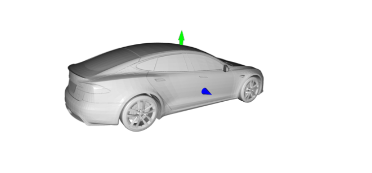

从上面的可视化中，我们看到这个汽车网格的方向如下：

XYZ 轴的原点：在汽车模型的体积中心（在上图中未显示，因为它位于汽车网格内部）。
X 轴（红色箭头）：沿着汽车的长度方向，正 X 轴指向汽车的引擎盖（上图中未显示，因为它位于汽车网格内部）。
Y 轴（绿色箭头）：沿着汽车的高度尺寸，正 Y 轴指向汽车的车顶。
Z 轴（蓝色箭头）：沿着汽车的宽度尺寸，正 Z 轴指向汽车的右侧。

现在让我们来看看这款车型的内部结构。为此，我们将在 Z 轴上裁剪网格并移除汽车的右半部分（正 Z 轴）。

# Cropping the car mesh using its bouding box to remove its right half (positive Z-axis).
bbox = mesh.get_axis_aligned_bounding_box()
bbox_points = np.asarray(bbox.get_box_points())
bbox_points[:, 2] = np.clip(bbox_points[:, 2], a_min=None, a_max=0)
bbox_cropped = o3d.geometry.AxisAlignedBoundingBox.create_from_points(o3d.utility.Vector3dVector(bbox_points))
mesh_cropped = mesh.crop(bbox_cropped)

# Visualizing the cropped mesh.
draw_geoms_list = [mesh_coord_frame, mesh_cropped]
o3d.visualization.draw_geometries(draw_geoms_list)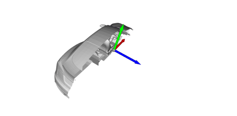

从上面的可视化图中，我们可以看到这款汽车模型拥有详细的内饰。现在我们已经看到了这个 3D 网格内部的内容，我们可以在移除属于汽车内部的“隐藏”点之前将其转换为点云。

2、通过采样点将网格转换为点云

通过定义我们希望从网格中采样的点数，可以在 Open3D 中轻松将网格转换为点云。

# Uniformly sampling 100,000 points from the mesh to convert it to a point cloud.
n_pts = 100_000
pcd = mesh.sample_points_uniformly(n_pts)

# Visualizing the point cloud.
draw_geoms_list = [mesh_coord_frame, pcd]
o3d.visualization.draw_geometries(draw_geoms_list)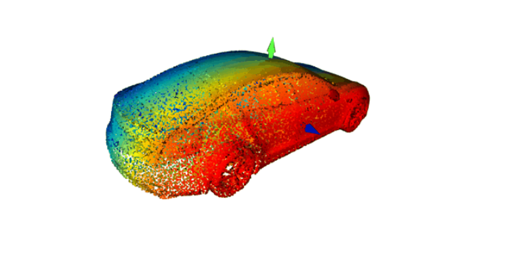

请注意，上面点云中的颜色仅表示点沿 Z 轴的位置。

如果我们像上面的网格一样裁剪点云，这就是它的样子：

# Cropping the car point cloud using bounding box to remove its right half (positive Z-axis).
pcd_cropped = pcd.crop(bbox_cropped)

# Visualizing the cropped point cloud.
draw_geoms_list = [mesh_coord_frame, pcd_cropped]
o3d.visualization.draw_geometries(draw_geoms_list)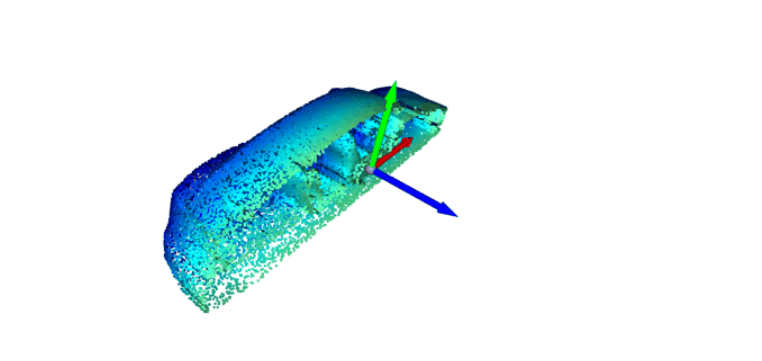

我们在裁剪点云的可视化中看到它还包含属于汽车模型内部的点。这是意料之中的，因为此点云是通过从整个网格中均匀采样点创建的。在下一节中，我们将移除这些属于汽车内部且不在点云外表面上的“隐藏”点。

3、从点云中移除隐藏点

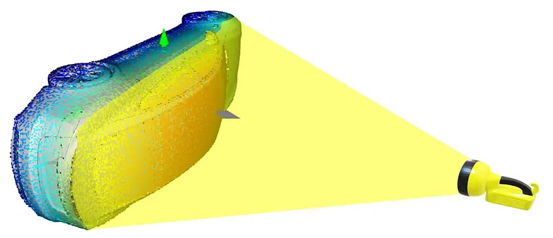
想象一下，你将一盏灯指向汽车模型的右侧。所有落在 3D 模型右外表面上的点都会被照亮，而点云中的所有其他点都不会。

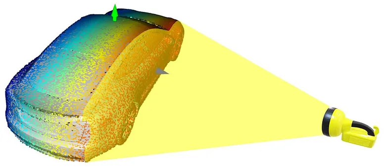
现在让我们将这些被照亮的点标记为“可见”，将所有未被照亮的点标记为“隐藏”。这些“隐藏”点还包括属于汽车内部的所有点。

此操作在 Open3D 中称为隐藏点移除（Hidden Point Removal）。为了使用 Open3D 在点云上执行此操作，请运行以下代码行：

# Defining the camera and radius parameters for the hidden point removal operation.
diameter = np.linalg.norm(np.asarray(pcd.get_min_bound()) - np.asarray(pcd.get_max_bound()))
camera = [0, 0, diameter]
radius = diameter * 100

# Performing the hidden point removal operation on the point cloud using the
# camera and radius parameters defined above.
# The output is a list of indexes of points that are visible.
_, pt_map = pcd.hidden_point_removal(camera, radius)

使用上面的可见点索引输出列表，我们可以在可视化点云之前用不同的颜色为可见点和隐藏点着色。

# Painting all the visible points in the point cloud in blue, and all the hidden points in red.

pcd_visible = pcd.select_by_index(pt_map)
pcd_visible.paint_uniform_color([0, 0, 1])    # Blue points are visible points (to be kept).
print("No. of visible points : ", pcd_visible)

pcd_hidden = pcd.select_by_index(pt_map, invert=True)
pcd_hidden.paint_uniform_color([1, 0, 0])    # Red points are hidden points (to be removed).
print("No. of hidden points : ", pcd_hidden)

# Visualizing the visible (blue) and hidden (red) points in the point cloud.
draw_geoms_list = [mesh_coord_frame, pcd_visible, pcd_hidden]
o3d.visualization.draw_geometries(draw_geoms_list)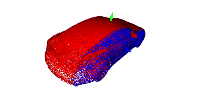

从上面的可视化中，我们可以看到隐藏点移除操作是如何从给定的相机视角进行的。该操作从给定的相机视点消除了被前景中的点遮挡的背景中的所有点。

为了更好地理解这一点，我们可以再次重复相同的操作，但这次是在稍微旋转点云之后。实际上，我们正在尝试改变这里的观点。但是我们不是通过重新定义相机参数来改变它，而是旋转点云本身。

# Defining a function to convert degrees to radians.
def deg2rad(deg):
    return deg * np.pi/180

# Rotating the point cloud about the X-axis by 90 degrees.
x_theta = deg2rad(90)
y_theta = deg2rad(0)
z_theta = deg2rad(0)
tmp_pcd_r = copy.deepcopy(pcd)
R = tmp_pcd_r.get_rotation_matrix_from_axis_angle([x_theta, y_theta, z_theta])
tmp_pcd_r.rotate(R, center=(0, 0, 0))

# Visualizing the rotated point cloud.
draw_geoms_list = [mesh_coord_frame, tmp_pcd_r]
o3d.visualization.draw_geometries(draw_geoms_list)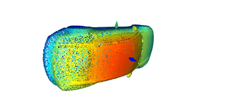

通过对旋转的汽车模型再次重复相同的过程，我们会看到这次落在 3D 模型（车顶）上部外表面上的所有点都会被照亮，而该点中的所有其他点云不会。

我们可以通过运行以下代码行对旋转后的点云重复隐藏点移除操作：

# Performing the hidden point removal operation on the rotated point cloud
# using the same camera and radius parameters defined above.
# The output is a list of indexes of points that are visible.
_, pt_map = tmp_pcd_r.hidden_point_removal(camera, radius)

# Painting all the visible points in the rotated point cloud in blue,
# and all the hidden points in red.

pcd_visible = tmp_pcd_r.select_by_index(pt_map)
pcd_visible.paint_uniform_color([0, 0, 1])    # Blue points are visible points (to be kept).
print("No. of visible points : ", pcd_visible)

pcd_hidden = tmp_pcd_r.select_by_index(pt_map, invert=True)
pcd_hidden.paint_uniform_color([1, 0, 0])    # Red points are hidden points (to be removed).
print("No. of hidden points : ", pcd_hidden)

# Visualizing the visible (blue) and hidden (red) points in the rotated point cloud.
draw_geoms_list = [mesh_coord_frame, pcd_visible, pcd_hidden]
o3d.visualization.draw_geometries(draw_geoms_list)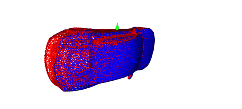

上面旋转点云的可视化清楚地说明了隐藏点移除操作的工作原理。所以现在，为了从这个汽车点云中移除所有“隐藏”点，我们可以依次执行这个隐藏点移除操作，方法是将点云围绕所有三个轴从 -90 度到 +90 度轻微旋转。在每次隐藏点移除操作之后，我们可以聚合点索引的输出列表。在所有隐藏点移除操作之后，聚合的点索引列表将包含所有未隐藏的点（即点云外表面上的点）。以下代码执行此顺序隐藏点删除操作：

# Defining a function to rotate a point cloud in X, Y and Z-axis.
def get_rotated_pcd(pcd, x_theta, y_theta, z_theta):
    pcd_rotated = copy.deepcopy(pcd)
    R = pcd_rotated.get_rotation_matrix_from_axis_angle([x_theta, y_theta, z_theta])
    pcd_rotated.rotate(R, center=(0, 0, 0))
    return pcd_rotated

# Defining a function to get the camera and radius parameters for the point cloud
# for the hidden point removal operation.
def get_hpr_camera_radius(pcd):
    diameter = np.linalg.norm(np.asarray(pcd.get_min_bound()) - np.asarray(pcd.get_max_bound()))
    camera = [0, 0, diameter]
    radius = diameter * 100
    return camera, radius

# Defining a function to perform the hidden point removal operation on the
# point cloud using the camera and radius parameters defined earlier.
# The output is a list of indexes of points that are not hidden.
def get_hpr_pt_map(pcd, camera, radius):
    _, pt_map = pcd.hidden_point_removal(camera, radius)    
    return pt_map

# Performing the hidden point removal operation sequentially by rotating the
# point cloud slightly in each of the three axes from -90 to +90 degrees,
# and aggregating the list of indexes of points that are not hidden after
# each operation.

# Defining a list to store the aggregated output lists from each hidden
# point removal operation.
pt_map_aggregated = []

# Defining the steps and range of angle values by which to rotate the point cloud.
theta_range = np.linspace(-90, 90, 7)

# Counting the number of sequential operations.
view_counter = 1
total_views = theta_range.shape[0] ** 3

# Obtaining the camera and radius parameters for the hidden point removal operation.
camera, radius = get_hpr_camera_radius(pcd)

# Looping through the angle values defined above for each axis.
for x_theta_deg in theta_range:
    for y_theta_deg in theta_range:
        for z_theta_deg in theta_range:

            print(f"Removing hidden points - processing view {view_counter} of {total_views}.")

            # Rotating the point cloud by the given angle values.
            x_theta = deg2rad(x_theta_deg)
            y_theta = deg2rad(y_theta_deg)
            z_theta = deg2rad(z_theta_deg)
            pcd_rotated = get_rotated_pcd(pcd, x_theta, y_theta, z_theta)
            
            # Performing the hidden point removal operation on the rotated
            # point cloud using the camera and radius parameters defined above.
            pt_map = get_hpr_pt_map(pcd_rotated, camera, radius)
            
            # Aggregating the output list of indexes of points that are not hidden.
            pt_map_aggregated += pt_map

            view_counter += 1

# Removing all the duplicated points from the aggregated list by converting it to a set.
pt_map_aggregated = list(set(pt_map_aggregated))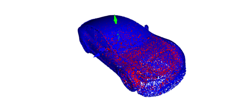

让我们再次裁剪点云，看看属于汽车内部的点。

# Cropping the point cloud of visible points using bounding box defined
# earlier to remove its right half (positive Z-axis).
pcd_visible_cropped = pcd_visible.crop(bbox_cropped)

# Cropping the point cloud of hidden points using bounding box defined
# earlier to remove its right half (positive Z-axis).
pcd_hidden_cropped = pcd_hidden.crop(bbox_cropped)

# Visualizing the cropped point clouds.
draw_geoms_list = [mesh_coord_frame, pcd_visible_cropped, pcd_hidden_cropped]
o3d.visualization.draw_geometries(draw_geoms_list)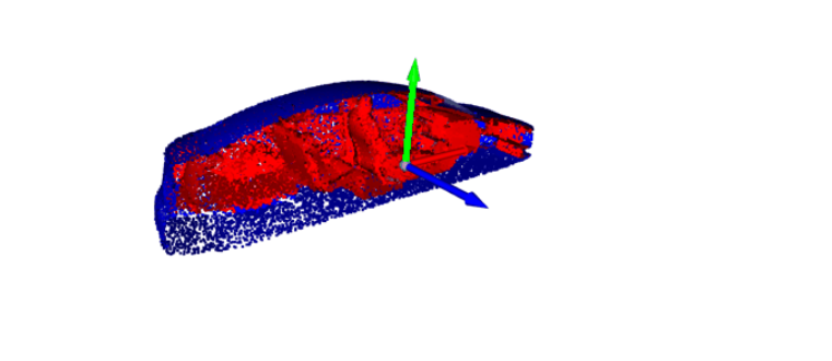

从上面隐藏点去除操作后裁剪点云的可视化，我们看到所有属于汽车模型内部的“隐藏”点（红色）现在都与“可见”点分开了点云的外表面（蓝色）。

4、将点云转换为数据帧

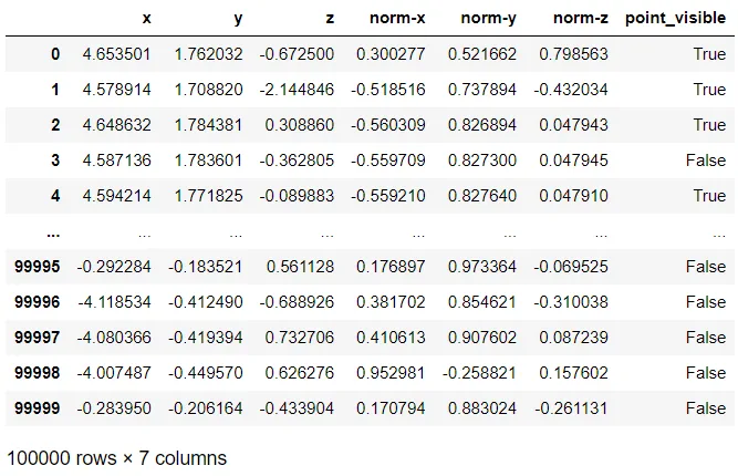
正如人们所预料的那样，点云中每个点的位置可以由三个数值定义——X、Y 和 Z 坐标。然而，回想一下在上一节中，我们还估计了 3D 网格中每个点的表面法线。当我们从这个网格中采样点来创建点云时，点云中的每个点还包含三个与这些表面法线相关的附加属性——X、Y 和 Z 方向上的法线单位矢量坐标。

因此，为了将点云转换为数据帧，点云中的每个点都可以由以下七个属性列表示在一行中：

X 坐标（float）
Y 坐标（float）
Z 坐标（float）
X方向的法向量坐标（float）
Y方向的法向量坐标（float）
Z方向的法向量坐标（float）
点可见（布尔值 True 或 False）

可以通过运行以下代码行将点云转换为数据帧（Data frame）：

# Creating a dataframe for the point cloud with the X, Y & Z positional coordinates
# and the normal unit vector coordinates in the X, Y & Z directions of all points.
pcd_df = pd.DataFrame(np.concatenate((np.asarray(pcd.points), np.asarray(pcd.normals)), axis=1),
                      columns=["x", "y", "z", "norm-x", "norm-y", "norm-z"]
                     )

# Adding a column to indicate whether the point is visible or not using the aggregated
# list of indexes of points from the hidden point removal operation above.
pcd_df["point_visible"] = False
pcd_df.loc[pt_map_aggregated, "point_visible"] = True

这将返回如下所示的数据框，其中每个点都是由上述七个属性列表示的一行。

5、保存点云和数据帧

现在可以通过运行以下代码行来保存点云（隐藏点移除前后）和数据帧：

# Saving the entire point cloud as a .pcd file.
pcd_save_path = "data/3d_model.pcd"
o3d.io.write_point_cloud(pcd_save_path, pcd)

# Saving the point cloud with the hidden points removed as a .pcd file.
pcd_visible_save_path = "data/3d_model_hpr.pcd"
o3d.io.write_point_cloud(pcd_visible_save_path, pcd_visible)

# Saving the point cloud dataframe as a .csv file.
pcd_df_save_path = "data/3d_model.csv"
pcd_df.to_csv(pcd_df_save_path, index=False)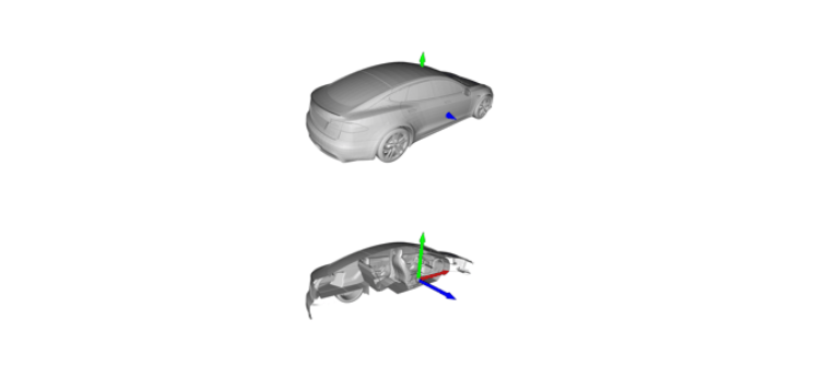

就是这样！希望这个教程让你对如何在 Python 中处理 3D 数据有所了解！

原文链接：3D Data Processing with Open3D

BimAnt翻译整理，转载请标明出处

Open3D模型处理实战

0、开发环境准备

1、加载 3D 模型并可视化

2、通过采样点将网格转换为点云

3、从点云中移除隐藏点

4、将点云转换为数据帧

5、保存点云和数据帧

admin

GIS中的3D分析

GemPy地质建模实战

0、开发环境准备

1、加载 3D 模型并可视化

2、通过采样点将网格转换为点云

3、从点云中移除隐藏点

4、将点云转换为数据帧

5、保存点云和数据帧

GIS中的3D分析

GemPy地质建模实战

You might also like...

You might also like...