3D数据的邻域分析

NSDT工具推荐： Three.js AI纹理开发包 - YOLO合成数据生成器 - GLTF/GLB在线编辑 - 3D模型格式在线转换 - 可编程3D场景编辑器 - REVIT导出3D模型插件 - 3D模型语义搜索引擎 - Three.js虚拟轴心开发包 - 3D模型在线减面 - STL模型在线切割

距离计算和邻域分析是理解网格和点云的形状、结构和特征的重要工具。 本文将使用三个最广泛使用的 Python 3D 数据分析库 — Open3D、PyVista 和 Vedo 来提取基于距离的信息、将其可视化并展示示例用例。 与往常一样，提供了所有代码以及使用的网格和点云数据。 谁说 3D 对象的邻域分析应该很困难？

1、内容简述

与深度图或体素相比，点云和网格表示 3D 空间中的非结构化数据。 点由它们的 (X, Y, Z) 坐标表示，在 3D 空间中可能彼此靠近的两个点在数组表示中可能很远。 点之间的距离也不相等，这意味着其中一些点可能紧密地聚集在一起或彼此远离。 这导致这样一个事实：与图像中的相同问题相比，理解某个点的邻域并不是一项简单的任务。

点之间的距离计算是点云和网格分析、噪声检测和去除、局部平滑和智能抽取模型等的重要组成部分。 距离计算也是 3D 深度学习模型不可或缺的一部分，既用于数据预处理，也是训练管道的一部分 [7]。 此外，经典的点云几何特征依赖于最近点的邻域计算和PCA分析[2, 8]。

特别是对于非常大的点云和复杂的网格，如果以暴力方式完成，所有点之间的距离的计算可能会变得非常资源密集且成本高昂。 我们将在本文中重点介绍的库使用 KD 树或八叉树的不同实现，将对象的 3D 空间划分为更易于管理和结构化的象限。 这样，这种分区可以完成一次，并且所有后续的距离查询都可以被加速和简化。 由于深入研究 KD 树和八叉树超出了本文的范围，因此我强烈建议你在深入研究所提供的示例之前观看这些 YouTube 视频 - 用于表示空间信息的多维数据 KdTree、四叉树和八叉树，尤其是 computerphile的k-d 树视频。

在本文中，我们还将简要介绍点云中点之间测地距离的计算。 该距离是连接图结构中两点之间的最短路径，其中我们计算点之间存在的边的数量。 这些距离可用于捕获有关 3D 对象的形状和点组成的信息，以及在处理 3D 表面的图形表示时。

在本文中，我们将仔细研究三个 Python 库——Open3D、PyVista 和 Vedo，以及它们生成 3D 网格和点云的邻域和邻接分析的功能。 选择这三个库是因为它们提供了简单易用的距离计算功能，可以在深度学习和处理管道中轻松实现。 这些库的功能也很齐全，并提供了网格和点云的分析和操作方法。 我们还将使用 SciPy 提供的 KD 树实现，因为它经过高度优化和并行化，使其在处理大型 3D 对象时非常有用。

为了演示点云和网格上的体素化，我使用了两个对象。 首先是 .ply 格式的鸭子雕像点云，其中包含每个点的 X、Y 和 Z 坐标，以及它们的 R、G 和 B 颜色，最后是 Nx、Ny 和 Nz 法线。 鸭子雕像是使用 Motion 摄影测量结构创建的，可免费用于商业、非商业、公共和私人项目。 该对象是较大数据集 [1] 的一部分，并已用于开发噪声检测和检查 [2] 以及尺度计算 [3] 的方法。 其次，使用著名的 .ply 格式的斯坦福兔子对象，因为它很容易获得并且广泛用于网格分析研究。 在引用适当的给定引文后，兔子可以自由用于非商业应用和研究[4]。

要学习这些教程，除了使用的库及其依赖项之外，你还需要 NumPy 和 SciPy。 所有代码都可以在 GitHub 存储库中找到。

2、使用 Open3D 进行邻域计算

Open3D 被认为是 3D 可视化 Python 库的标准，因为它包含点云、网格、深度图以及图形分析和可视化的方法。 它可以在 Linux、Mac 和 Windows 上轻松设置和运行，它包含一个名为 Open3D-ML 的专用于深度学习的完整分支，并具有用于 3D 重建的内置方法。

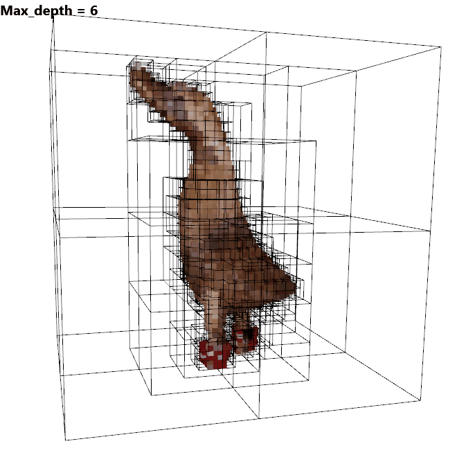
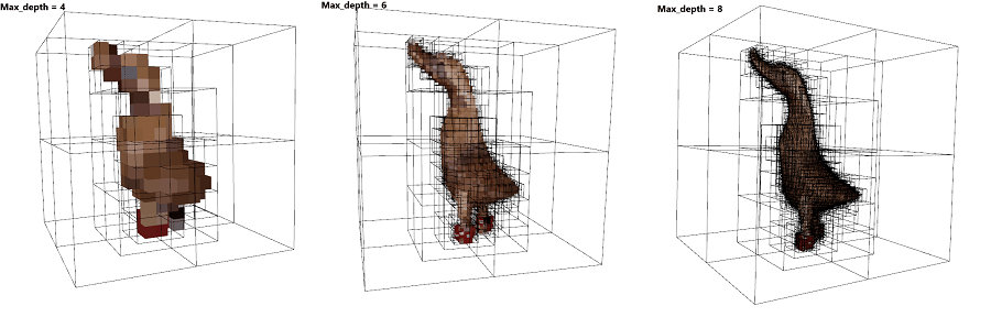
Open3D 包含直接从点云或体素网格构建八叉树的现成方法。 首先使用 open3d.geometry.Octree(max_depth=maximum_depth_of_the_struct) 初始化八叉树，然后使用方法 name_of_octree.convert_from_pointcloud(name_of_point_cloud) 直接从点云生成八叉树。 该方法隐式继承了点云的颜色信息。 下面显示了不同深度的八叉树以及简单的代码。

import open3d as o3d
import os

curr_max_depth = 8

point_cloud_path = os.path.join('point_cloud','duckStatue.ply')
point_cloud = o3d.io.read_point_cloud(point_cloud_path)

octree = o3d.geometry.Octree(max_depth = curr_max_depth)
octree.convert_from_point_cloud(point_cloud)
o3d.visualization.draw_geometries([octree])

一旦生成八叉树，就可以使用遍历和将为每个节点处理的函数来遍历它，并且可以在找到所需信息时提前停止。 此外，八叉树还具有以下功能：

• 定位一个点属于哪个叶节点— locate_leaf_node()
• 向特定节点插入新点 — insert_point()
• 查找树的根节点 — root_node

Open3D 还包含基于使用 FLANN [5] 构建的 KD 树的距离计算方法，也可以在此处找到不同绑定的方法。

首先使用函数 open3d.geometry.KDTreeFlann(name_of_3d_object) 从点云或网格生成 KD 树。 然后可以使用树来搜索许多用例。

首先，如果需要特定点的 K 最近邻，则可以调用函数 search_knn_vector_3d 以及要查找的邻居数量。 其次，如果需要特定半径内某个点周围的邻居，则可以与要搜索的半径的大小一起调用函数 search_radius_vector_3d 。最后，如果我们需要限制也在特定半径内的最近邻居的数量 ，可以调用函数 search_hybrid_vector_3d，它结合了前两个函数的标准。

这些函数还有一个更高维度的变体，用于使用例如 search_knn_vector_xd() 搜索维度高于 3 的邻居，其中维度需要手动设置为输入。 KD 树本身是一次性预先计算的，但搜索查询是一次针对单个点完成的。

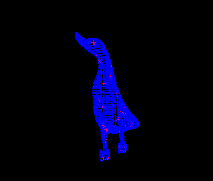
为了可视化查找点云中点的邻居的过程，我们将使用 LineSet() 结构，该结构采用多个节点和边并构造一个图结构。 为此，我们首先将鸭子雕像点云加载为 Open3D 点云，并对它进行二次采样以便于可视化。 为此，我们使用 voxel_down_sample() 内置函数。 然后我们计算下采样点云的 KD 树。 为了更好地可视化距离的计算方式，我们首先初始化可视化器对象，将背景更改为黑色，然后仅绘制点云。 最后，我们使用 register_animation_callback()注册一个动画回调函数。 下面的代码显示了此初始设置。

# Load point cloud .ply into Open3D point cloud object
point_cloud_path = os.path.join('point_cloud','duckStatue.ply')
point_cloud = o3d.io.read_point_cloud(point_cloud_path)

# Downsample the point cloud using voxel downsampling
point_cloud = point_cloud.voxel_down_sample(voxel_size=0.02)

# get the points and colors as separate numpy arrays
points = np.asarray(point_cloud.points)
colors = np.asarray(point_cloud.colors)

# Calculate the KDTree from the point cloud
pcd_tree = o3d.geometry.KDTreeFlann(point_cloud)

# Recolor the point cloud in blue, just to get a better contrast with the distance lines
point_cloud.paint_uniform_color([0, 0, 1])

# Initialize a visualizer object
vis = o3d.visualization.Visualizer()
# Create a window, name it and scale it
vis.create_window(window_name='Duck Visualize', width=800, height=600)

# Set background color to black
opt = vis.get_render_option()
opt.background_color = np.asarray([0, 0, 0])

# Add the point cloud to the visualizer
vis.add_geometry(point_cloud)

# Register a new animation callback function
vis.register_animation_callback(build_edges)

# Run the visualizater
vis.run()
# Once the visualizer is closed destroy the window and clean up
vis.destroy_window()

初始设置完成后，可以为每个更新周期调用回调函数并生成每个点的邻域。 为点云中的每个点调用函数 search_knn_vector_3d ，并指定所需的 k 个最近邻点的数量。 该函数返回点的数量、点的索引以及点本身。 为了生成线段，我们采用找到的邻居点以及从中心点到每个邻居的边缘数组。 我们知道，只有 k 个找到的邻居，我们生成边缘数组作为每个邻居的中心索引和边缘索引的相同堆栈。 创建的 LineSet 将添加到主 LineSet 对象中，并且几何图形和渲染器将被更新。 一旦遍历完所有点，就会通过调用 clear()重置 LineSet。 下面给出了回调函数的代码。

# Params class containing the counter and the main LineSet object holding all line subsets
class params():

    counter = 0
    full_line_set = o3d.geometry.LineSet()

# Callback function for generating the LineSets from each neighborhood
def build_edges(vis):
    # Run this part for each point in the point cloud
    if params.counter < len(points):
        # Find the K-nearest neighbors for the current point. In our case we use 6
        [k, idx, _] = pcd_tree.search_knn_vector_3d(points[params.counter,:], 6)
        # Get the neighbor points from the indices
        points_temp = points[idx,:]
        
        # Create the neighbours indices for the edge array
        neighbours_num = np.arange(len(points_temp))
        # Create a temp array for the center point indices
        point_temp_num = np.zeros(len(points_temp))
        # Create the edges array as a stack from the current point index array and the neighbor indices array
        edges = np.vstack((point_temp_num,neighbours_num)).T

        # Create a LineSet object and give it the points as nodes together with the edges
        line_set = o3d.geometry.LineSet()
        line_set.points = o3d.utility.Vector3dVector(points_temp)
        line_set.lines = o3d.utility.Vector2iVector(edges)
        # Color the lines by either using red color for easier visualization or with the colors from the point cloud
        line_set.paint_uniform_color([1, 0, 0])
        # line_set.paint_uniform_color(colors[params.counter,:])
        
        # Add the current LineSet to the main LineSet
        params.full_line_set+=line_set
        
        # if the counter just started add the LineSet geometry
        if params.counter==0:
            vis.add_geometry(params.full_line_set)
        # else update the geometry 
        else:
            vis.update_geometry(params.full_line_set)
        # update the render and counter
        vis.update_renderer()
        params.counter +=1
    else:
        # if the all point have been used reset the counter and clear the lines
        params.counter=0
        params.full_line_set.clear()

现在我们已经了解了如何使用 Open3D 中的内置函数计算 KD 树，我们将扩展这个概念。 我们研究了如何使用 3D 点坐标之间的距离，但我们也可以在其他空间上工作。 鸭子雕像带有点云中每个点的计算法线和颜色。 我们可以使用这些特征以相同的方式构建 KD 树，并探索这些特征空间中点之间的关系。

除了为这些功能构建 KD 树之外，我们还将使用 SciPy 中预先构建的函数，只是为了探索生成数据的替代方法。 构建 KD 树是通过 SciPy 的空间部分完成的。 为了构建它们，我们可以调用 scipy.spatial.KDTree(chosen_metric)。 一旦我们有了树结构，我们就可以调用 name_of_tree.query(array_points_to_query, k = number_of_neighbours)。 这与 Open3D 实现不同，在 Open3D 实现中我们可以一次查询单个点的最近点。 当然，这意味着通过 SciPy 实现，我们可以使用高度优化的函数来预先计算所有距离，这对于加快后续计算很有用。 查询函数的输出是两个数组——每个查询点的最近点距离和最近点的索引，格式为 N x k，其中 N 是查询点的数量，k 是邻居的数量。

所有其他功能与前面的示例相同，但为了更清晰的演示，我们将每个步骤分成一个函数：

我们对点云进行下采样：

# Downsampling function, using the voxel down sampling from Open3D, which inputs a point cloud and outputs arrays containing points, colors, normals
# There is no checks to see if the point cloud has colors and normals so either ensure that your point cloud has them or add normal and pseudo color generation
def downsample(point_cloud, voxel_size=0.02):
    point_cloud = point_cloud.voxel_down_sample(voxel_size=voxel_size)
    points = np.asarray(point_cloud.points)
    colors = np.asarray(point_cloud.colors)
    normals = np.asarray(point_cloud.normals)

    return points,colors,normals

我们计算 KD 树和点之间的边：

# Function to calculate KD-tree, closest neighbourhoods and edges between the points
def calculate_edges(metric, num_neighbours = 4):
    # Calculate the KD-tree of the selected feature space
    tree = KDTree(metric)
    # Query the neighbourhoods for each point of the selected feature space to each point
    d_kdtree, idx = tree.query(metric,k=num_neighbours)
    # Remove the first point in the neighbourhood as this is just the queried point itself
    idx= idx[:,1:]

    # Create the edges array between all the points and their closest neighbours
    point_numbers = np.arange(len(metric))
    # Repeat each point in the point numbers array the number of closest neighbours -> 1,2,3,4... becomes 1,1,1,1,2,2,2,2,3,3,3,3,4,4,4,4...
    point_numbers = np.repeat(point_numbers, num_neighbours-1)
    # Flatten  the neighbour indices array -> from [1,3,10,14], [4,7,17,23], ... becomes [1,3,10,4,7,17,23,...]
    idx_flatten = idx.flatten()
    # Create the edges array by combining the two other ones as a vertical stack and transposing them to get the input that LineSet requires
    edges = np.vstack((point_numbers,idx_flatten)).T

    return edges

我们构建一个 LineSet并输出点云以进行可视化，最后创建一个可视化对象并显示所有内容。

# Create Open3D objects to contain the LineSet and output Point cloud for visualization purposes 
def build_objects(points,colors,edges):
    line_set = o3d.geometry.LineSet()
    line_set.points = o3d.utility.Vector3dVector(points)
    line_set.lines = o3d.utility.Vector2iVector(edges)
    line_set.paint_uniform_color([1, 0, 0])

    point_cloud = o3d.geometry.PointCloud()
    point_cloud.points = o3d.utility.Vector3dVector(points)
    point_cloud.colors = o3d.utility.Vector3dVector(colors)

    return line_set, point_cloud

# Create the visualizer object, set the background to black and create a coordinate system.
# Add the output point cloud and line set
def visualize_objects( line_set, point_cloud, plot_description ):
    # Initialize a visualizer object
    vis = o3d.visualization.Visualizer()
    # Create a window, name it and scale it
    vis.create_window(window_name = plot_description, width=800, height=600)
    opt = vis.get_render_option()
    opt.background_color = np.asarray([0, 0, 0])

    vis.add_geometry(point_cloud)
    vis.add_geometry(line_set)
    # Create a coordinate frame, set its size and origin position
    mesh_frame = o3d.geometry.TriangleMesh.create_coordinate_frame(
    size=0.6,origin=(-1,-1,-1))
    vis.add_geometry(mesh_frame)
    # We run the visualizater
    vis.run()
    # Once the visualizer is closed destroy the window and clean up
    vis.destroy_window()

最后，我们可以选择计算邻域并可视化不同的特征空间。 下面显示了这些示例，其中显示了坐标、法线和颜色空间中可视化的坐标、法线和颜色的邻域。

if __name__ == '__main__':

    # Load point cloud .ply into Open3D point cloud object
    point_cloud_path = os.path.join('point_cloud','duckStatue.ply')
    point_cloud_input = o3d.io.read_point_cloud(point_cloud_path)

    # Downsample
    points,colors,normals = downsample(point_cloud_input)
    # Calculate KD-tree / Edges - here you can change points to colors or normals to calculate their neighborhoods
    edges = calculate_edges(points, num_neighbours= 4)
    # Build objects - here you can change the points to normals or colors to show different features spaces and you can change the colors to color the feature space differently
    line_set, point_cloud_output = build_objects(points,colors,edges)
    # Visualzie objects
    visualize_objects(line_set,point_cloud_output,'Point Cloud with Distance Graph')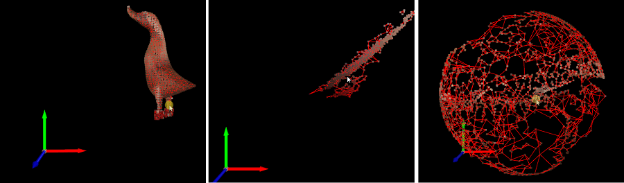

3、使用 PyVista 进行邻域计算

PyVista 是一个功能齐全的库，用于点云、网格和数据集的分析、操作和可视化。 它构建在 VTK 之上，提供简单的开箱即用功能。 PyVista 可用于创建具有多个绘图、屏幕、小部件和动画的交互式应用程序。 它可用于生成 3D 表面、分析网格结构、消除噪声和转换数据。

PyVista 包含许多现成的函数，用于对点和顶点进行分组、计算邻域以及查找最近的点。 PyVista 中最简单的功能之一是使用 VTK 的连通性过滤器对点进行分组，并根据距离和连通性标准（例如共享顶点、法线方向之间的距离、颜色等）提取连通单元。可以通过调用 name_of_3d_object.connectivity()。 这将返回一个标量数组，其中包含每个点的区域 ID。

另外，如果我们在连接函数调用中添加 largest=True，我们就可以直接得到最大的连通区域。 我们可以通过 add_mesh_threshold(3d_object_name) 将这些连接区域 ID 与 PyVista 中内置的交互式阈值功能结合起来，以便能够可视化和提取所需的区域。 下面给出了此操作的代码。

import pyvista as pv 
import os
# Read the duck statue point cloud
pc_path = os.path.join('point_cloud','duckStatue.ply')
pc = pv.read(pc_path) 

# Use the connectivity filter to get the scalar array of region ids
conn = pc.connectivity(largest=False)
# See the active scalar fields in the calculated object
print(conn.active_scalars_name)
# Show the ids
print(conn["RegionId"])
# Set up a plotter
p = pv.Plotter()
# add the interactive thresholding tool and show everything
p.add_mesh_threshold(conn,show_edges=True)
p.show()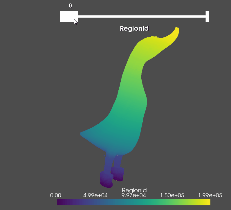

除此之外，PyVista 还具有内置的邻域和最近点计算功能。 这是通过 find_closest_point(point_to_query, n = number_of_neighbors) 函数完成的，其中可以给出单个点作为输入，以及要返回的邻域的大小。 该函数返回输入附近的点的索引。 该函数与 Open3D 函数具有相同的限制，即一次只能计算一个点的一个邻域。 在需要完成大量点的情况下，SciPy 实现速度更快、更优化。 PyVista 的 API 参考中也提到了这一点。

为了演示 find_closest_point 功能并在 PyVista 的用例中为其提供更多上下文，我们将动画演示鸭雕像点云的重建，一次一个点邻域。 这可以用作创建抽取函数、邻域分析函数等的基础。 我们还将整个事情整齐地打包在一个类中，以便可以轻松调用。

为了生成第二个点云并可视化当前点及其邻域，我们利用 PyVista 通过名称跟踪添加到绘图仪的对象这一事实。 我们将所有内容绘制为每次更新交互时调用的回调函数。 要更好地了解动画回调和网格更新的工作原理，你可以查看数据可视化和网格体素化文章。

import pyvista as pv
from pyvistaqt import BackgroundPlotter
import os
import numpy as np

# Class on building a replica point cloud one point neighbourhood at a time. 
class find_neighbours():
    def __init__(self,pc_points, num_neighbours):
        # Setup initial variables - get the point cloud, set a counter for the current point selected, getting the neighborhood
        # setup a array of booleans to keep track of the points that have been already checked and setting up the plotter
        self.pc_points = pc_points
        self.counter = 0
        self.num_neighbours = num_neighbours
        self.checked = np.zeros(len(pc_points), dtype=bool)
        self.p = BackgroundPlotter()


    # Update function called by the callback
    def every_point_neighborhood(self):
        # get the current point to calculate the neighborhood of
        point = pc_points[self.counter,:]
        # get all the indices of the neighbors of the current point
        index = pc.find_closest_point(point,self.num_neighbours)
        # get the neighbor points
        neighbours = pc_points[index,:]
        # mark the points as checked and extract the checked sub-point cloud
        self.checked[index] = True

        new_pc = pc_points[self.checked]
        # move the reconstructed point cloud in X direction so it can be more easier seen
        new_pc[:,0]+=1
        # add the neighborhood points, the center point and the new checked point clouds to the plotter.
        # Because we are using the same names PyVista knows to update the already existing ones
        self.p.add_mesh(neighbours, color="r", name='neighbors', point_size=8.0, render_points_as_spheres=True)
        self.p.add_mesh(point, color="b", name='center', point_size=10.0, render_points_as_spheres=True)
        self.p.add_mesh(new_pc, color="g", name='new_pc', render_points_as_spheres=True)
        # move the counter with a 100 points so the visualization is faster - change this to 1 to get all points
        self.counter+=100
        # get the point count
        pc_count = len(pc_points)
        # check if all points have been done. If yes then 0 the counter and the checked array
        if self.counter >= pc_count:
            self.counter = 0
            self.checked = np.zeros(len(pc_points), dtype=bool)

        # We update the whole plotter
        self.p.update()
    # visualization function
    def visualize_neighbours(self):
        # add the colored mesh of the duck statue. We set the RGB color scalar array as color by calling rgb=True
        self.p.add_mesh(pc, render_points_as_spheres=True, rgb=True)
        # We set the callback function and an interval of 100 between update cycles
        self.p.add_callback(self.every_point_neighborhood, interval=100)
        self.p.show()
        self.p.app.exec_()
        
if __name__ == '__main__':
    # Read the duck statue point cloud
    pc_path = os.path.join('point_cloud','duckStatue.ply')
    pc = pv.read(pc_path) 
    pc_points = pc.points
    pc_points = np.array(pc_points)

    neighbours_class = find_neighbours(pc_points, 400)
    neighbours_class.visualize_neighbours()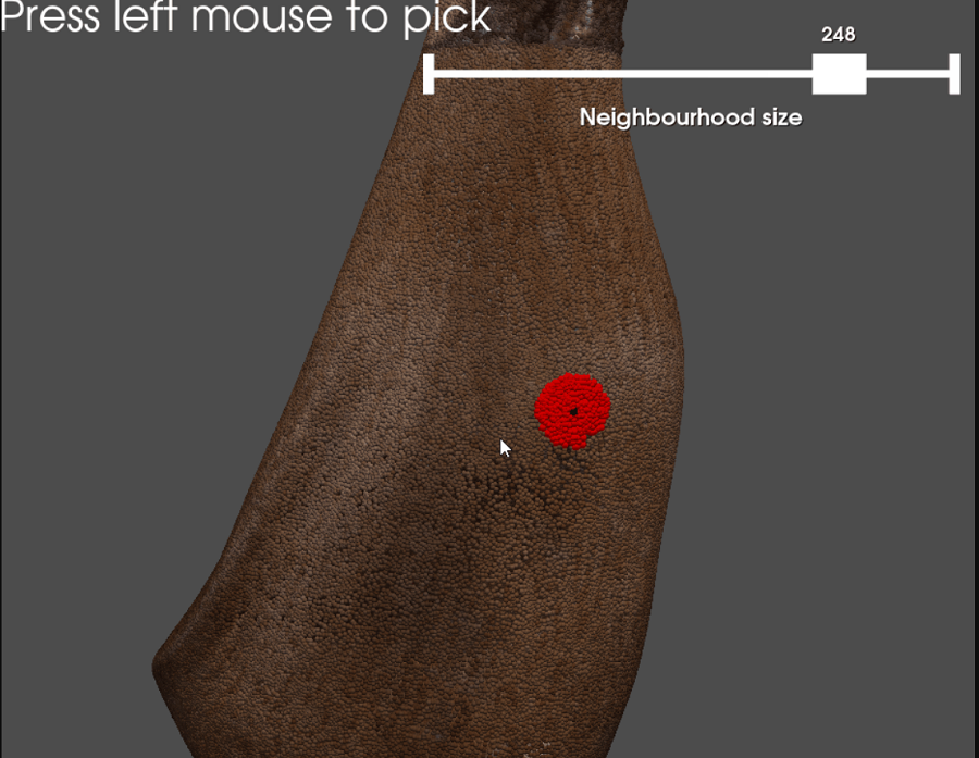

最后，我们可以展示如何将使用 find_closest_point() 的邻域计算与创建小部件和捕获鼠标事件的可能性结合起来。 我们将创建一个应用程序，可以检测用户在点云上单击的点并计算其邻居。 找到的邻居数量将根据滑块小部件进行选择。

使用 enable_point_picking()来选择点。 在此函数中，我们需要提供回调，并使用 show_message 输入设置将在屏幕上显示的消息，并能够使用 left_clicking=True 直接单击鼠标左键。

# Callback function for selecting points with the mouse
def manipulate_picked(point):
    # Get selected point and switch the boolean for having selected something to True
    params.point = point
    params.point_selected = True
    # Get the closest points indices 
    index = pc.find_closest_point(point,params.size)
    # Get the points themselves
    neighbours = pc_points[index,:]
    # add points representing the neighborhood and the selected point to the plotter
    p.add_mesh(neighbours, color="r", name='neighbors', point_size=8.0, render_points_as_spheres=True)
    p.add_mesh(point, color="b", name='center', point_size=10.0, render_points_as_spheres=True)

为了设置滑块小部件，我们使用 add_slider_widget 方法，并设置回调函数，以及滑块的最小值和最大值以及事件类型。 回调要做的唯一事情是获取滑块的新值，然后如果选择了该点，则调用函数来计算最近的点并可视化它们。

# Callback function for the slider widget for changing the neighborhood size 
def change_neighborhood(value):
    # change the slider value to int
    params.size = int(value)
    # call the point selection function if a point has already been selected
    if params.point_selected:
        manipulate_picked(params.point)

    return

这两个函数都设置为回调，并创建一个简单的参数类来跟踪所有共享变量。

# Class of parameters used in the two callback function
class params():
    # size of the neighborhood 
    size = 20
    # the selected point
    point = np.zeros([1,3])
    # is the point selected or not
    point_selected = False

pc_path = os.path.join('point_cloud','duckStatue.ply')
pc = pv.read(pc_path) 
# Initialize the plotter
p = pv.Plotter()
# Add the main duck statue point cloud as spheres and with colors 
p.add_mesh(pc, render_points_as_spheres=True, rgb=True)
# Initialize the mouse point picker callback and the slider widget callback
p.enable_point_picking(callback=manipulate_picked,show_message="Press left mouse to pick", left_clicking=True)
p.add_slider_widget(change_neighborhood, [10, 300], 20, title='Neighbourhood size', event_type = "always")
p.show()

4、使用 Vedo 进行邻域和距离计算

Vedo 是一个强大的 3D 对象科学可视化和分析库。 它具有用于处理点云、网格和 3D 体积的内置函数。 它可用于创建物理模拟，例如 2D 和 3D 对象运动、光学模拟、气体和液体流动模拟以及运动学等。 它包含功能齐全的 2D 和 3D 绘图界面，以及注释、动画和交互选项。 它可以用来可视化直方图、图表、密度图、时间序列等。它构建在VTK之上，与PyVista相同，可以在Linux、Mac和Windows上使用。

Vedo 具有开箱即用的功能，可通过函数 closestPoint() 查找给定半径内的所有最近点或k 最近邻点。 它与点一起在网格或点云上调用，需要找到其邻居以及半径或多个邻居。 在内部，该函数调用 VTK的 vtkPointLocator 对象，该对象用于通过将点周围的空间区域划分为矩形桶并查找落在每个桶中的点来快速定位 3D 空间中的点。 该方法被认为比 KD 树和八叉树慢，因此对于较大的点云，首选 SciPy 实现。

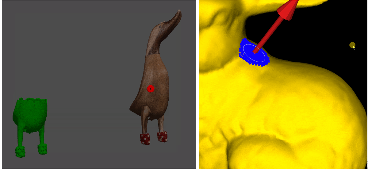
为了演示 Vedo 中邻域检测的工作原理，我们将创建一个简单的示例，其中用户单击网格以选择顶点并计算邻域。 我们将通过展示如何使用它来计算邻域的平均法线并为其拟合一个圆来扩展它。 这个简单的示例可以扩展用于拟合其他基元，如球体或平面，并可用于计算局部邻域特征、智能去噪、抽取和孔填充。 对于这些示例，我们将使用斯坦福兔子网格。

我们将使用函数 vedo.fitCircle(neighbourhood_points_array) 来拟合圆，然后通过使用 vedo.Circle() 生成圆和使用 vedo.Arrow() 生成法向量来可视化它。 我们通过调用 plot_name.addCallback('LeftButtonPress', name_of_callback_function)来实现鼠标点击回调。

# Callback function for selecting a point, calculating its neighborhood, calculating the average normal and fitting a circle to the neighborhood
def fit_circle(evt):
    # Check if anything has been clicked on
    if evt['actor'] != None:
        # From the event get the 3D point that has been selected
        params.point = evt['picked3d']

        # Find all the indices of points in a radius around the clicked point
        closets_ids = mesh.closestPoint(params.point, radius = 0.01, returnPointId = True)
        all_points = mesh.points()
        # get the neighbor points
        closets_points = all_points[closets_ids,:]
        # get their normals
        closets_normals = mesh.normals()
        closets_normals = closets_normals[closets_ids,:]
        # Calculate the average normal of the neighborhood
        closets_normals_avg = closets_normals.mean(axis=0)
    
        # Make the selected point and its neighborhood into Vedo point clouds
        center_point = vedo.Points([params.point], r=20).color("red")
        neighbourhood = vedo.Points(closets_points, r=10).color("blue")
        # Fit a circle to the neighborhood points and return the circle center, radius and normal or orientation
        (center_circle, radius, normal_to_circle) = vedo.fitCircle(closets_points)
        # Create a circle 3D object, make into a wireframe and orient it based on the circle normal
        circle = vedo.Circle(center_circle, r=radius).wireframe().orientation(normal_to_circle)
        # Create a end point for the array object showing the average normal - 0.05 is a scaling factor
        end_point = params.point + closets_normals_avg*0.05
        # Make an arrow object
        arrow = vedo.Arrow(startPoint=params.point, endPoint=end_point, c='red')
        # Check if t he created objects in the Plotter are equil to 5, if they are remove them
        if len(plt.actors)==5:
            for i in range(0,4): plt.pop()
        # add the new created objects
        plt.add(center_point, neighbourhood, circle, arrow)

这里需要提到的是，对于回调函数，我们首先检查是否有使用 event['actor'] 选择的对象，然后如果有对象，则使用 event['picked3d'] 获取所选点。 每次我们删除所有代表中心点、邻近点、圆圈和箭头的旧角色并构建新的角色。

另一个可以从 Vedo 直接计算的有趣距离度量是测地距离。 测地距离是 3D 对象的流形或曲面上的点之间的最短距离或路径。 这非常类似于平面上点之间的直线。 测地距离是分段平滑曲线，积分时是给定点之间的最短路径。 测地距离对于计算球体或球面空间中的点之间的距离非常有用，它用于测量地球上点之间的最短距离。 从更简单的角度来看，如果我们将测地距离与欧几里德距离进行比较，测地线会考虑点所在表面的基本形状，而欧几里德则不会。

在 Vedo 中，有一个名为 name_of_mesh.geodesic() 的现成函数，用于计算网格上两个给定点之间的距离。 要求是网格是水密的并且没有任何几何缺陷。 该函数返回一个由两点之间的所有边组成的路径对象。 它使用 Dijkstra 算法来寻找最短路径，其实现基于 [6] 中描述的算法，如 VTK 的类描述中所述。

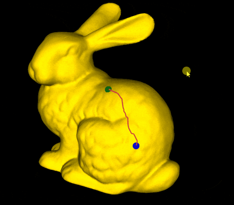
我们将通过创建一个交互式测地路径计算示例来利用这一点，其中用户在 3D 网格上选择两个点，并且它们之间的路径被可视化。 为此，我们将再次使用方法 addCallback('LeftButtonPress') 以及一个列表来保留选定的点，并在每次新单击时添加和删除它们。 下面给出了此操作的代码。

# Callback function for calculating the geodesic distance between two selected points
def calculate_geodesic(evt):
    # Check if the click has selected a object
    if evt['actor'] != None:
        # Get the 3D point from the selected object
        params.points_list.append(evt['picked3d'])
        # if there are more than 2 points in the point list remove the first one
        if len(params.points_list) > 2:
            params.points_list.pop(0)
        # if there are exactly 2 points calculate the geodesic distance between them and visualize the path
        if len(params.points_list) == 2:
            # get point 1 and point 2 from the list
            point_1 = params.points_list[0]
            point_2 = params.points_list[1]

            print(point_1, point_2)
            # Calculate the geodesic distance and get the path in red color
            path = mesh.geodesic(point_1, point_2).c("red4")
            # Make two point clouds representing the first and second points in different colors 
            p1 = vedo.Points([point_1], r=20).color("blue")
            p2 = vedo.Points([point_2], r=20).color("green")
            # if there are more than 4 objects remove the old 3 ones
            if len(plt.actors)==4:
                for i in range(0,3): plt.pop()
            # add the new ones
            plt.add(path, p1, p2)

        # render
        plt.render()

5、结束语

网格和点云的距离和邻域计算可以成为分析其表面、检测缺陷、噪声和感兴趣区域的极其强大的工具。 基于邻域计算局部特征是智能 3D 对象抽取、重新拓扑、水印和平滑的一部分。 计算每个点的 K 最近邻是从点云生成图、体素化和曲面构建的重要部分。 最后，许多处理 3D 对象的深度学习模型需要计算点邻域和最近点距离。 通过本文，我们展示了可以在 Python 中快速轻松地计算此信息。 我们还展示了可以在 Python 中创建基于距离计算的交互式应用程序和动画，而无需牺牲可用性。 我们还展示了如何计算不同深度的 KD 树和八叉树。

现在我们知道如何计算点邻域，下一步是从中提取局部特征和表面信息。 在下一篇文章中，我们将介绍用于特征提取的 Python 库——基于 PCA 的特征提取和几何特征提取。

原文链接：Neighborhood Analysis, KD-Trees, and Octrees for Meshes and Point Clouds in Python

BimAnt翻译整理，转载请标明出处